


变化的长模型#
import arviz as az
import bambi as bmb
import matplotlib.pyplot as plt
import numpy as np
import pandas as pd
import preliz as pz
import pymc as pm
import statsmodels.api as sm
import xarray as xr

lowess = sm.nonparametric.lowess
%config InlineBackend.figure_format = 'retina'  # high resolution figures
az.style.use("arviz-darkgrid")
rng = np.random.default_rng(42)
对变化的研究涉及同时分析个体变化的轨迹,并从所研究的个体集合中抽象出更广泛的关于所讨论变化性质的见解。因此,很容易因为专注于树木而忽略了森林。在这个例子中,我们将展示使用分层贝叶斯模型研究个体群体内变化的一些微妙之处——从个体内部视角转向个体间/跨个体视角。
我们将遵循Singer和Willett在《应用纵向数据分析》中概述的模型构建讨论和迭代方法。更多详情请参见Singer .D和Willett .B [2003])。我们将与他们的展示有所不同,因为他们专注于使用最大似然法拟合数据,而我们将使用PyMC和贝叶斯方法。在这一方法中,我们遵循了Solomon Kurz在brms中的工作,参见Kurz [2021]。我们强烈推荐这两本书,以获得对这里讨论问题的更详细介绍。
演示文稿的结构#
青少年酒精消费随时间变化分析
插曲:使用Bambi的替代模型规范
青少年外化行为随时间变化分析
结论
探索性数据分析:个体差异的混乱#
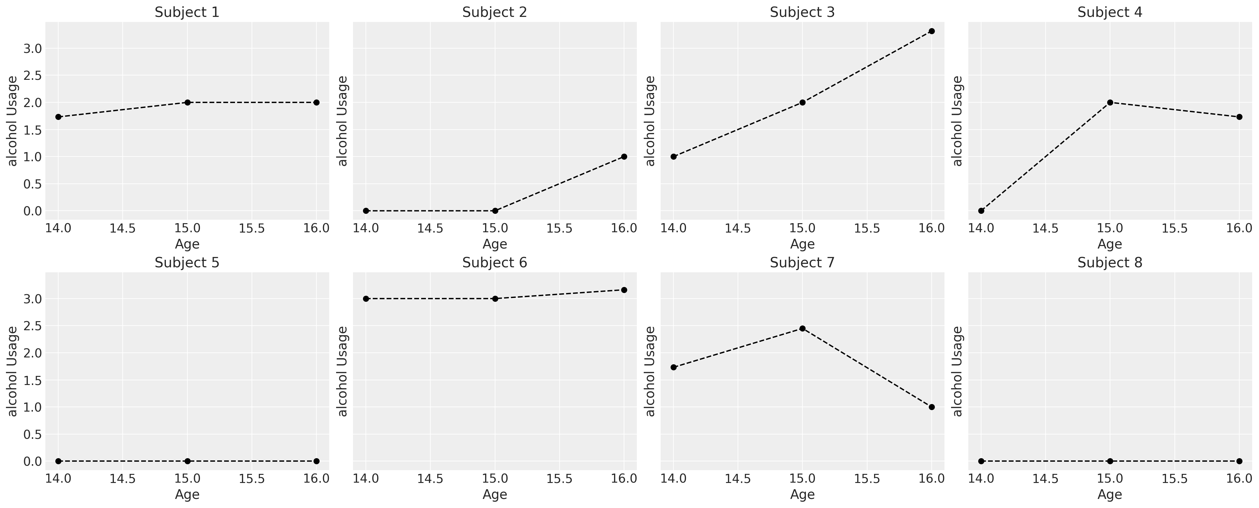
对于任何纵向分析,我们需要三个组成部分:(1) 多次数据收集 (2) 合适的时间定义 (3) 一个感兴趣的结果。结合这些,我们可以评估个体在时间上的变化与该结果的关系。在这个模型的第一系列中,我们将研究青少年酒精使用情况如何随着从14岁开始每年收集的数据在儿童之间变化。
try:
    df = pd.read_csv("../data/alcohol1_pp.csv")
except FileNotFoundError:
    df = pd.read_csv(pm.get_data("alcohol1_pp.csv"))

df["peer_hi_lo"] = np.where(df["peer"] > df["peer"].mean(), 1, 0)
df
| id | age | coa | male | age_14 | alcuse | peer | cpeer | ccoa | peer_hi_lo | |
|---|---|---|---|---|---|---|---|---|---|---|
| 0 | 1 | 14 | 1 | 0 | 0 | 1.732051 | 1.264911 | 0.246911 | 0.549 | 1 |
| 1 | 1 | 15 | 1 | 0 | 1 | 2.000000 | 1.264911 | 0.246911 | 0.549 | 1 |
| 2 | 1 | 16 | 1 | 0 | 2 | 2.000000 | 1.264911 | 0.246911 | 0.549 | 1 |
| 3 | 2 | 14 | 1 | 1 | 0 | 0.000000 | 0.894427 | -0.123573 | 0.549 | 0 |
| 4 | 2 | 15 | 1 | 1 | 1 | 0.000000 | 0.894427 | -0.123573 | 0.549 | 0 |
| ... | ... | ... | ... | ... | ... | ... | ... | ... | ... | ... |
| 241 | 81 | 15 | 0 | 1 | 1 | 0.000000 | 1.549193 | 0.531193 | -0.451 | 1 |
| 242 | 81 | 16 | 0 | 1 | 2 | 0.000000 | 1.549193 | 0.531193 | -0.451 | 1 |
| 243 | 82 | 14 | 0 | 0 | 0 | 0.000000 | 2.190890 | 1.172890 | -0.451 | 1 |
| 244 | 82 | 15 | 0 | 0 | 1 | 1.414214 | 2.190890 | 1.172890 | -0.451 | 1 |
| 245 | 82 | 16 | 0 | 0 | 2 | 1.000000 | 2.190890 | 1.172890 | -0.451 | 1 |
246 行 × 10 列
首先,我们将研究一部分儿童的消费模式,以了解他们报告的使用情况如何表现出不同的轨迹。所有这些轨迹都可以合理地建模为线性现象。
fig, axs = plt.subplots(2, 4, figsize=(20, 8), sharey=True)
axs = axs.flatten()
for i, ax in zip(df["id"].unique()[0:8], axs):
    temp = df[df["id"] == i].sort_values("age")
    ax.plot(temp["age"], temp["alcuse"], "--o", color="black")
    ax.set_title(f"Subject {i}")
    ax.set_ylabel("alcohol Usage")
    ax.set_xlabel("Age")
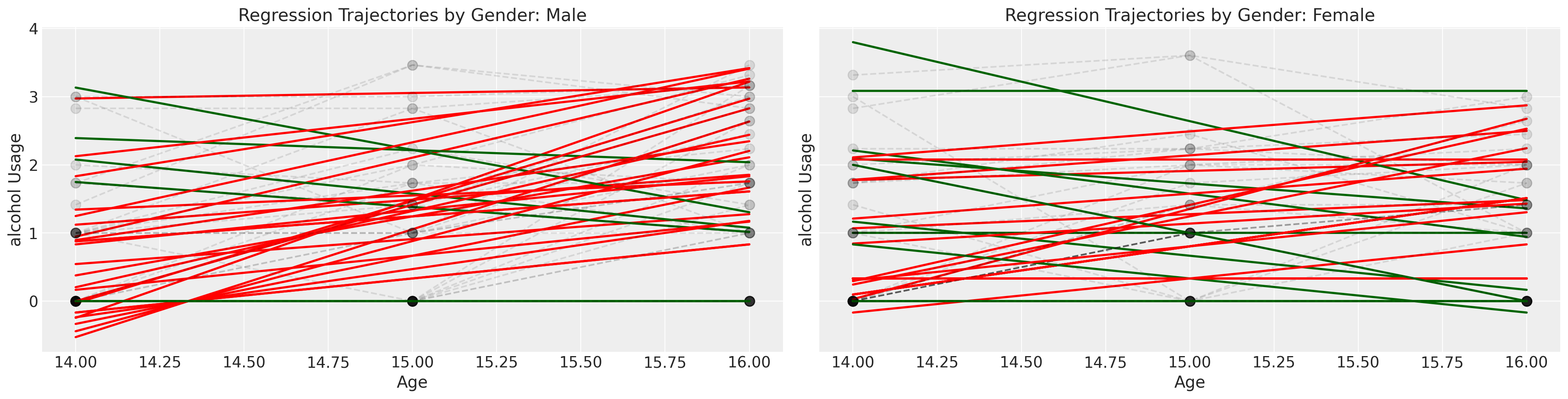
我们可能会认为酒精使用模式因性别的影响而有所不同,但个体的轨迹是嘈杂的。在接下来的系列图中,我们在个体数据上拟合了简单的回归模型,并根据斜率系数是\(\color{green}{负的}\)还是\(\color{red}{正的}\)来为趋势线着色。这非常粗略地给出了每个性别的个体消费模式是否以及如何变化的印象。
绿色和红色的线代表个人的OLS拟合,但灰色虚线代表个人的观察轨迹。
Show code cell source
fig, axs = plt.subplots(1, 2, figsize=(20, 5), sharey=True)
lkup = {0: "Male", 1: "Female"}

axs = axs.flatten()
for i in df["id"].unique():
    temp = df[df["id"] == i].sort_values("age")
    params = np.polyfit(temp["age"], temp["alcuse"], 1)
    positive_slope = params[0] > 0
    if temp["male"].values[0] == 1:
        index = 0
    else:
        index = 1
    if positive_slope:
        color = "red"
    else:
        color = "darkgreen"
    y = params[0] * temp["age"] + params[1]
    axs[index].plot(temp["age"], y, "-", color=color, linewidth=2)
    axs[index].plot(
        temp["age"], temp["alcuse"], "--o", mec="black", alpha=0.1, markersize=9, color="black"
    )
    axs[index].set_title(f"Regression Trajectories by Gender: {lkup[index]}")
    axs[index].set_ylabel("alcohol Usage")
    axs[index].set_xlabel("Age")
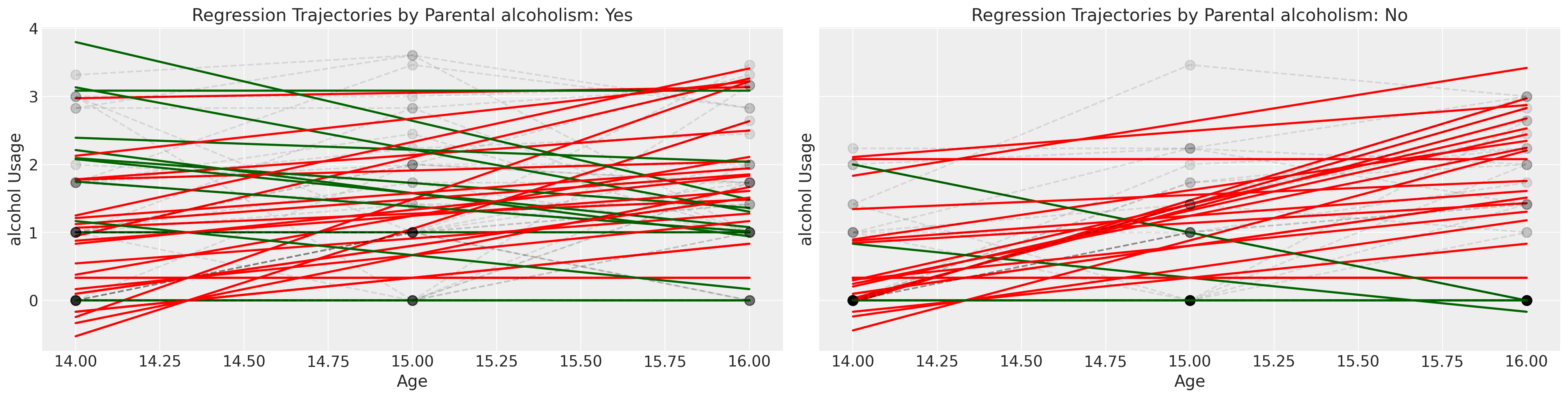
接下来我们检查相同的图表,但根据孩子是否是酗酒父母的子女进行分层。
Show code cell source
fig, axs = plt.subplots(1, 2, figsize=(20, 5), sharey=True)
lkup = {0: "Yes", 1: "No"}
axs = axs.flatten()
for i in df["id"].unique():
    temp = df[df["id"] == i].sort_values("age")
    params = np.polyfit(temp["age"], temp["alcuse"], 1)
    positive_slope = params[0] > 0
    if temp["coa"].values[0] == 1:
        index = 0
    else:
        index = 1
    if positive_slope:
        color = "red"
    else:
        color = "darkgreen"
    y = params[0] * temp["age"] + params[1]
    axs[index].plot(temp["age"], y, "-", color=color, linewidth=2)
    axs[index].plot(
        temp["age"], temp["alcuse"], "--o", alpha=0.1, mec="black", markersize=9, color="black"
    )
    axs[index].set_title(f"Regression Trajectories by Parental alcoholism: {lkup[index]}")
    axs[index].set_ylabel("alcohol Usage")
    axs[index].set_xlabel("Age")
我们将通过粗略地将孩子们分为他们的同伴群体是否报告了高酒精使用得分来结束对这个数据集的探索。
Show code cell source
fig, axs = plt.subplots(1, 2, figsize=(20, 5), sharey=True)
lkup = {0: "Hi", 1: "Lo"}
axs = axs.flatten()
for i in df["id"].unique():
    temp = df[df["id"] == i].sort_values("age")
    params = np.polyfit(temp["age"], temp["alcuse"], 1)
    positive_slope = params[0] > 0
    if temp["peer_hi_lo"].values[0] == 1:
        index = 0
    else:
        index = 1
    if positive_slope:
        color = "red"
    else:
        color = "darkgreen"
    y = params[0] * temp["age"] + params[1]
    axs[index].plot(temp["age"], y, "-", color=color, label="Regression Fit")
    axs[index].plot(
        temp["age"],
        temp["alcuse"],
        "--o",
        mec="black",
        alpha=0.1,
        markersize=9,
        color="black",
        label="Observed",
    )
    axs[index].set_title(f"Regression Trajectories by Peer Usage Score: {lkup[index]}")
    axs[index].set_ylabel("alcohol Usage")
    axs[index].set_xlabel("Age")
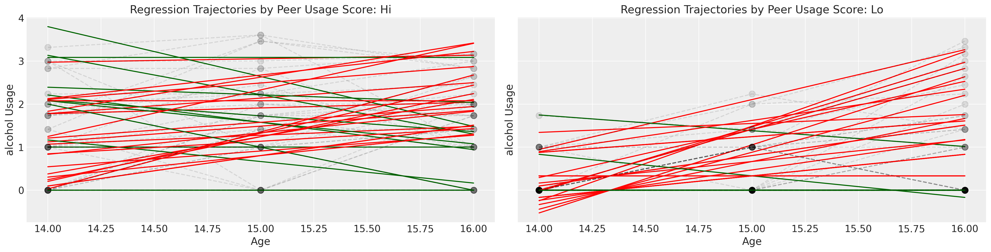
这次探索性练习的整体印象是巩固复杂性的概念。虽然有许多个体的轨迹和独特的时间旅程,但如果我们想对感兴趣的现象——父母酗酒对子女饮酒行为的影响——做出一般性的陈述,我们需要做的不仅仅是面对复杂性而放弃。
随时间变化的建模#
我们从简单的无条件模型开始,该模型仅模拟个体对最终结果的贡献。换句话说,该模型的特点是它不包含任何预测因子。它用于划分结果中的变异来源,根据个体偏离总体均值的程度,将或多或少异常的行为归因于每个个体。
无条件均值模型#
id_indx, unique_ids = pd.factorize(df["id"])
coords = {"ids": unique_ids, "obs": range(len(df["alcuse"]))}
with pm.Model(coords=coords) as model:
    subject_intercept_sigma = pm.HalfNormal("subject_intercept_sigma", 2)
    subject_intercept = pm.Normal("subject_intercept", 0, subject_intercept_sigma, dims="ids")
    global_sigma = pm.HalfStudentT("global_sigma", 1, 3)
    global_intercept = pm.Normal("global_intercept", 0, 1)
    grand_mean = pm.Deterministic("grand_mean", global_intercept + subject_intercept[id_indx])
    outcome = pm.Normal("outcome", grand_mean, global_sigma, observed=df["alcuse"], dims="obs")
    idata_m0 = pm.sample_prior_predictive()
    idata_m0.extend(
        pm.sample(random_seed=100, target_accept=0.95, idata_kwargs={"log_likelihood": True})
    )
    idata_m0.extend(pm.sample_posterior_predictive(idata_m0))

pm.model_to_graphviz(model)
Sampling: [global_intercept, global_sigma, outcome, subject_intercept, subject_intercept_sigma]
Auto-assigning NUTS sampler...
Initializing NUTS using jitter+adapt_diag...
Multiprocess sampling (4 chains in 4 jobs)
NUTS: [subject_intercept_sigma, subject_intercept, global_sigma, global_intercept]
Sampling 4 chains for 1_000 tune and 1_000 draw iterations (4_000 + 4_000 draws total) took 5 seconds.
Sampling: [outcome]

az.summary(idata_m0, var_names=["subject_intercept_sigma", "global_intercept", "global_sigma"])
| mean | sd | hdi_3% | hdi_97% | mcse_mean | mcse_sd | ess_bulk | ess_tail | r_hat | |
|---|---|---|---|---|---|---|---|---|---|
| subject_intercept_sigma | 0.766 | 0.084 | 0.604 | 0.917 | 0.002 | 0.001 | 2852.0 | 2579.0 | 1.0 |
| global_intercept | 0.913 | 0.100 | 0.709 | 1.088 | 0.003 | 0.002 | 1032.0 | 1798.0 | 1.0 |
| global_sigma | 0.757 | 0.043 | 0.676 | 0.833 | 0.001 | 0.001 | 3442.0 | 2960.0 | 1.0 |
fig, ax = plt.subplots(figsize=(20, 7))
expected_individual_mean = idata_m0.posterior["subject_intercept"].mean(axis=1).values[0]

ax.bar(
    range(len(expected_individual_mean)),
    np.sort(expected_individual_mean),
    color="slateblue",
    ec="black",
)
ax.set_xlabel("Individual ID")
ax.set_ylabel("alcohol Use")
ax.set_title("Distribution of Individual Modifications to the Grand Mean");
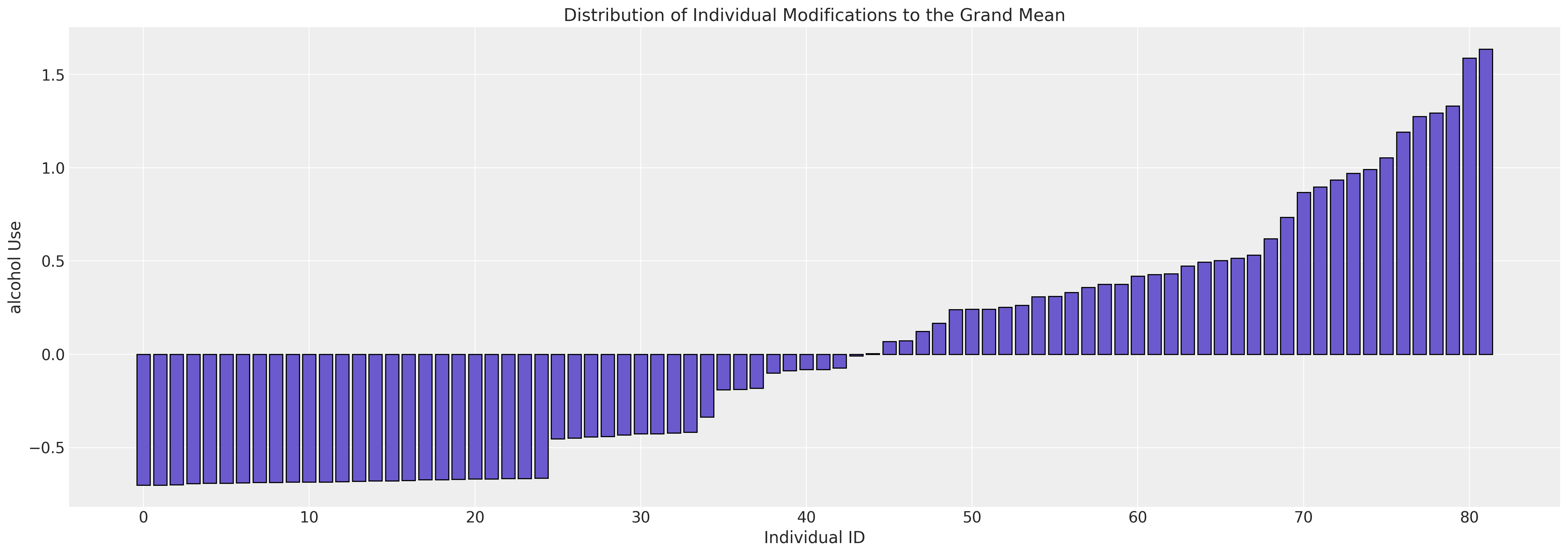
我们在这里看到研究中每个个体对总体均值隐含修正的变化。
无条件增长模型#
接下来,我们将更明确地建模个体对回归模型斜率的贡献,其中时间是关键预测因子。这个模型的结构值得停下来考虑。在不同的领域和学科中,这种层次模型有各种不同的实例。经济学、政治学、心理测量学和生态学都有自己稍微不同的词汇来命名模型的各个部分:固定效应、随机效应、内部估计量、外部估计量……等等,这个列表还在继续,讨论也因此变得复杂。这些术语是模糊的,并且使用方式各不相同。Wilett 和 Singer 提到了 Level 1 和 Level 2 子模型,但精确的术语并不重要。
这些模型中重要的是层次结构。存在一个全局现象和一个特定主题的现象实例化。该模型允许我们将全局模型与每个主题的个体贡献组合起来。这有助于模型解释主题层面的未观察到的异质性。根据模型规范,每个主题的斜率和截距可能会有所不同。它不能解决所有形式的偏差,但它确实有助于解释模型预测中的这种偏斜来源。
拟合模型后,我们不仅了解到每个个体如何修改全局模型,还让我们学习到全局参数。特别是,我们允许对表示时间的变量系数进行特定主题的修改。对于我们在接下来的一系列模型中概述的所有层次模型,都存在一种广泛相似的组合模式。在贝叶斯设置中,我们试图学习最适合数据的参数。在PyMC中实现模型的代码如下:
id_indx, unique_ids = pd.factorize(df["id"])
coords = {"ids": unique_ids, "obs": range(len(df["alcuse"]))}
with pm.Model(coords=coords) as model:
    age_14 = pm.MutableData("age_14_data", df["age_14"].values)

    ## Level 1
    global_intercept = pm.Normal("global_intercept", 0, 1)
    global_sigma = pm.HalfStudentT("global_sigma", 1, 3)
    global_age_beta = pm.Normal("global_age_beta", 0, 1)

    subject_intercept_sigma = pm.HalfNormal("subject_intercept_sigma", 5)
    subject_age_sigma = pm.HalfNormal("subject_age_sigma", 5)

    ## Level 2
    subject_intercept = pm.Normal("subject_intercept", 0, subject_intercept_sigma, dims="ids")
    subject_age_beta = pm.Normal("subject_age_beta", 0, subject_age_sigma, dims="ids")

    growth_model = pm.Deterministic(
        "growth_model",
        (global_intercept + subject_intercept[id_indx])
        + (global_age_beta + subject_age_beta[id_indx]) * age_14,
    )
    outcome = pm.Normal(
        "outcome", growth_model, global_sigma, observed=df["alcuse"].values, dims="obs"
    )
    idata_m1 = pm.sample_prior_predictive()
    idata_m1.extend(
        pm.sample(random_seed=100, target_accept=0.95, idata_kwargs={"log_likelihood": True})
    )
    idata_m1.extend(pm.sample_posterior_predictive(idata_m1))

pm.model_to_graphviz(model)
/home/osvaldo/proyectos/00_BM/pymc-devs/pymc/pymc/data.py:304: FutureWarning: MutableData is deprecated. All Data variables are now mutable. Use Data instead.
  warnings.warn(
Sampling: [global_age_beta, global_intercept, global_sigma, outcome, subject_age_beta, subject_age_sigma, subject_intercept, subject_intercept_sigma]
Auto-assigning NUTS sampler...
Initializing NUTS using jitter+adapt_diag...
Multiprocess sampling (4 chains in 4 jobs)
NUTS: [global_intercept, global_sigma, global_age_beta, subject_intercept_sigma, subject_age_sigma, subject_intercept, subject_age_beta]
Sampling 4 chains for 1_000 tune and 1_000 draw iterations (4_000 + 4_000 draws total) took 13 seconds.
Sampling: [outcome]

西格玛项(方差分量)可能是理解模型中最重要的部分。全局和特定于主题的西格玛项代表了我们在模型中允许的变异来源。全局效应可以被认为是整个人群中的“固定”效应,而特定于主题的项则是从同一个人群中“随机”抽取的。
az.summary(
    idata_m1,
    var_names=[
        "global_intercept",
        "global_sigma",
        "global_age_beta",
        "subject_intercept_sigma",
        "subject_age_sigma",
    ],
)
| mean | sd | hdi_3% | hdi_97% | mcse_mean | mcse_sd | ess_bulk | ess_tail | r_hat | |
|---|---|---|---|---|---|---|---|---|---|
| global_intercept | 0.644 | 0.103 | 0.441 | 0.830 | 0.002 | 0.002 | 2100.0 | 2584.0 | 1.00 |
| global_sigma | 0.612 | 0.045 | 0.526 | 0.696 | 0.001 | 0.001 | 1293.0 | 2791.0 | 1.00 |
| global_age_beta | 0.271 | 0.062 | 0.158 | 0.389 | 0.001 | 0.001 | 4585.0 | 3257.0 | 1.00 |
| subject_intercept_sigma | 0.754 | 0.084 | 0.597 | 0.909 | 0.001 | 0.001 | 3178.0 | 3130.0 | 1.00 |
| subject_age_sigma | 0.347 | 0.069 | 0.217 | 0.477 | 0.003 | 0.002 | 694.0 | 1058.0 | 1.01 |
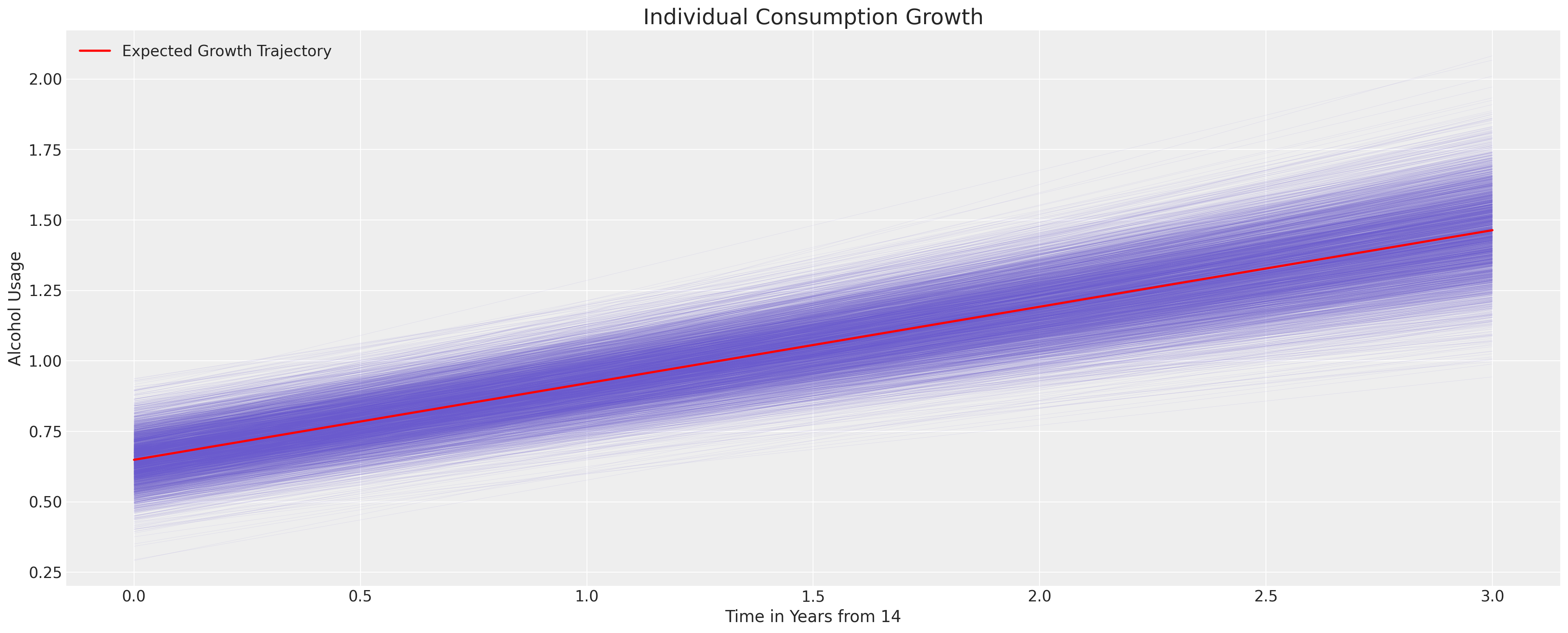
我们现在可以通过使用后验分布来推导隐含模型的不确定性。我们通过在所有受试者中取平均参数估计值来绘制推导出的轨迹。下面我们将看到如何在我们关注个体成长时,改为关注受试者内的估计。这里我们的关注点是青少年酒精使用的一般隐含轨迹。
fig, ax = plt.subplots(figsize=(20, 8))
posterior = az.extract(idata_m1.posterior)
intercept_group_specific = posterior["subject_intercept"].mean(dim="ids")
slope_group_specific = posterior["subject_age_beta"].mean(dim="ids")
a = posterior["global_intercept"].mean() + intercept_group_specific
b = posterior["global_age_beta"].mean() + slope_group_specific
time_xi = xr.DataArray(np.arange(4))
ax.plot(time_xi, (a + b * time_xi).T, color="slateblue", alpha=0.2, linewidth=0.2)
ax.plot(
    time_xi, (a.mean() + b.mean() * time_xi), color="red", lw=2, label="Expected Growth Trajectory"
)
ax.set_ylabel("Alcohol Usage")
ax.set_xlabel("Time in Years from 14")
ax.legend()
ax.set_title("Individual Consumption Growth", fontsize=20);
父母酗酒的失控影响#
接下来,我们将添加第二个预测变量及其与年龄的交互作用来修改结果。这扩展了上述模型,如下所示:
id_indx, unique_ids = pd.factorize(df["id"])
coords = {"ids": unique_ids, "obs": range(len(df["alcuse"]))}
with pm.Model(coords=coords) as model:
    age_14 = pm.MutableData("age_14_data", df["age_14"].values)
    coa = pm.MutableData("coa_data", df["coa"].values)

    ## Level 1
    global_intercept = pm.Normal("global_intercept", 0, 1)
    global_sigma = pm.HalfStudentT("global_sigma", 1, 3)
    global_age_beta = pm.Normal("global_age_beta", 0, 1)
    global_coa_beta = pm.Normal("global_coa_beta", 0, 1)
    global_coa_age_beta = pm.Normal("global_coa_age_beta", 0, 1)

    subject_intercept_sigma = pm.HalfNormal("subject_intercept_sigma", 5)
    subject_age_sigma = pm.HalfNormal("subject_age_sigma", 5)

    ## Level 2
    subject_intercept = pm.Normal("subject_intercept", 0, subject_intercept_sigma, dims="ids")
    subject_age_beta = pm.Normal("subject_age_beta", 0, subject_age_sigma, dims="ids")

    growth_model = pm.Deterministic(
        "growth_model",
        (global_intercept + subject_intercept[id_indx])
        + global_coa_beta * coa
        + global_coa_age_beta * (coa * age_14)
        + (global_age_beta + subject_age_beta[id_indx]) * age_14,
    )
    outcome = pm.Normal(
        "outcome", growth_model, global_sigma, observed=df["alcuse"].values, dims="obs"
    )
    idata_m2 = pm.sample_prior_predictive()
    idata_m2.extend(
        pm.sample(random_seed=100, target_accept=0.95, idata_kwargs={"log_likelihood": True})
    )
    idata_m2.extend(pm.sample_posterior_predictive(idata_m2))

pm.model_to_graphviz(model)
/home/osvaldo/proyectos/00_BM/pymc-devs/pymc/pymc/data.py:304: FutureWarning: MutableData is deprecated. All Data variables are now mutable. Use Data instead.
  warnings.warn(
Sampling: [global_age_beta, global_coa_age_beta, global_coa_beta, global_intercept, global_sigma, outcome, subject_age_beta, subject_age_sigma, subject_intercept, subject_intercept_sigma]
Auto-assigning NUTS sampler...
Initializing NUTS using jitter+adapt_diag...
Multiprocess sampling (4 chains in 4 jobs)
NUTS: [global_intercept, global_sigma, global_age_beta, global_coa_beta, global_coa_age_beta, subject_intercept_sigma, subject_age_sigma, subject_intercept, subject_age_beta]
Sampling 4 chains for 1_000 tune and 1_000 draw iterations (4_000 + 4_000 draws total) took 16 seconds.
Sampling: [outcome]

az.summary(
    idata_m2,
    var_names=[
        "global_intercept",
        "global_sigma",
        "global_age_beta",
        "global_coa_age_beta",
        "subject_intercept_sigma",
        "subject_age_sigma",
    ],
    stat_focus="median",
)
| median | mad | eti_3% | eti_97% | mcse_median | ess_median | ess_tail | r_hat | |
|---|---|---|---|---|---|---|---|---|
| global_intercept | 0.320 | 0.087 | 0.088 | 0.565 | 0.004 | 2284.281 | 2552.0 | 1.00 |
| global_sigma | 0.613 | 0.030 | 0.537 | 0.705 | 0.002 | 1577.315 | 2186.0 | 1.01 |
| global_age_beta | 0.290 | 0.057 | 0.129 | 0.449 | 0.002 | 2820.643 | 2815.0 | 1.00 |
| global_coa_age_beta | -0.046 | 0.081 | -0.268 | 0.182 | 0.003 | 2861.193 | 2935.0 | 1.00 |
| subject_intercept_sigma | 0.663 | 0.054 | 0.524 | 0.814 | 0.002 | 2662.958 | 2366.0 | 1.00 |
| subject_age_sigma | 0.351 | 0.045 | 0.215 | 0.469 | 0.002 | 1046.679 | 752.0 | 1.01 |
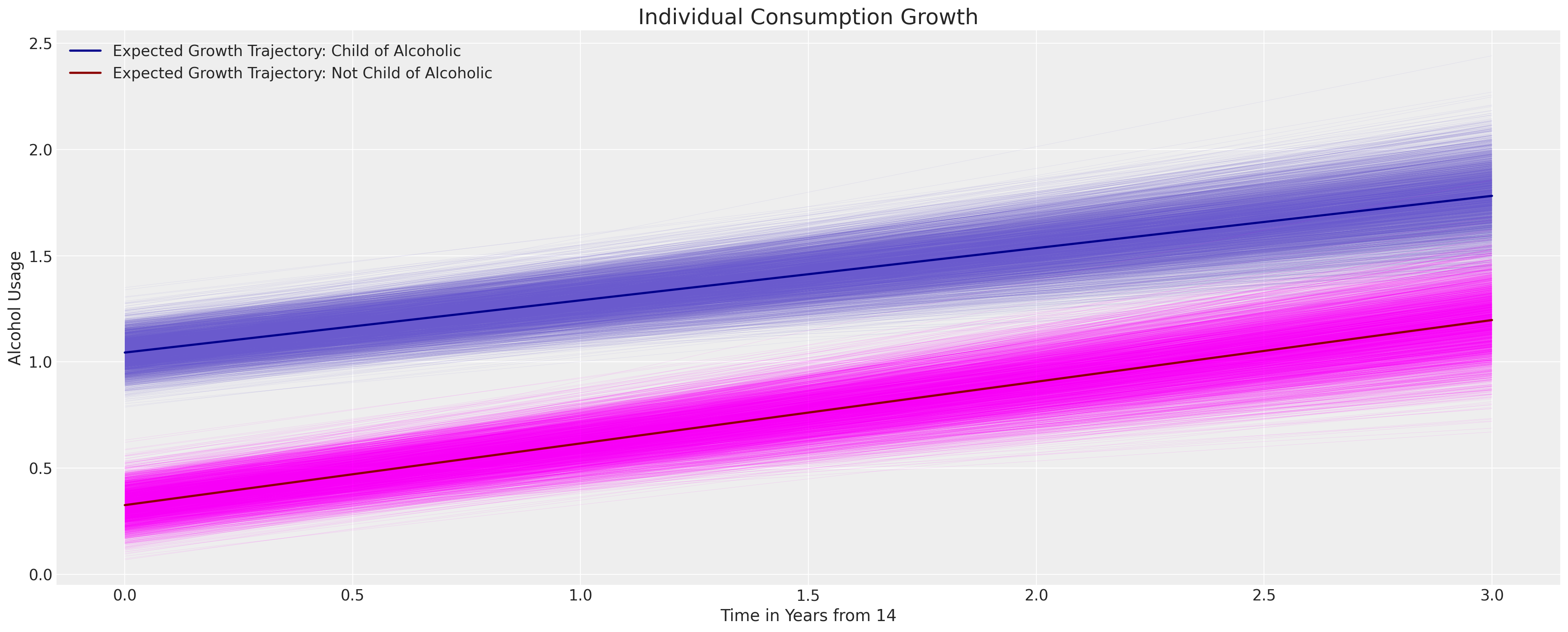
我们可以看到,这里包含的父母酗酒的二元标志对儿童消费的增长轨迹没有显著影响,但它确实改变了截距项的可能位置。
fig, ax = plt.subplots(figsize=(20, 8))
posterior = az.extract(idata_m2.posterior)
intercept_group_specific = posterior["subject_intercept"].mean(dim="ids")
slope_group_specific = posterior["subject_age_beta"].mean(dim="ids")
a = posterior["global_intercept"].mean() + intercept_group_specific
b = posterior["global_age_beta"].mean() + slope_group_specific
b_coa = posterior["global_coa_beta"].mean()
b_coa_age = posterior["global_coa_age_beta"].mean()

time_xi = xr.DataArray(np.arange(4))
ax.plot(
    time_xi,
    (a + b * time_xi + b_coa * 1 + b_coa_age * (time_xi * 1)).T,
    color="slateblue",
    linewidth=0.2,
    alpha=0.2,
)
ax.plot(
    time_xi,
    (a + b * time_xi + b_coa * 0 + b_coa_age * (time_xi * 0)).T,
    color="magenta",
    linewidth=0.2,
    alpha=0.2,
)
ax.plot(
    time_xi,
    (a.mean() + b.mean() * time_xi + b_coa * 1 + b_coa_age * (time_xi * 1)),
    color="darkblue",
    lw=2,
    label="Expected Growth Trajectory: Child of Alcoholic",
)
ax.plot(
    time_xi,
    (a.mean() + b.mean() * time_xi + b_coa * 0 + b_coa_age * (time_xi * 0)),
    color="darkred",
    lw=2,
    label="Expected Growth Trajectory: Not Child of Alcoholic",
)
ax.set_ylabel("Alcohol Usage")
ax.set_xlabel("Time in Years from 14")
ax.legend()
ax.set_title("Individual Consumption Growth", fontsize=20);
这已经暗示了分层纵向模型如何允许我们探讨政策问题和因果干预的影响。政策转变或特定干预在隐含的增长轨迹中的影响可能会导致重大的投资决策。然而,我们将这些评论作为暗示,因为关于在面板数据设计中使用因果推断的文献丰富且存在争议。差异中的差异文献充满了关于有意义地解释因果问题所需条件的警告。例如,参见差异中的差异以获取更多讨论和相关辩论的参考。一个关键点是,虽然主题级别的术语有助于解释数据中的一种异质性,但它们无法解释所有来源的个体变异,尤其是与时间相关的变异。
我们将暂时忽略因果推断的细微差别,接下来考虑同伴效应的引入如何改变我们模型所隐含的关联。
控制同伴效应的模型#
为了解释性和简化我们的采样器,我们将同龄人数据围绕其均值进行中心化。同样,这个模型自然地使用这些控制因素及其与年龄这一焦点变量的交互项来指定。
id_indx, unique_ids = pd.factorize(df["id"])
coords = {"ids": unique_ids, "obs": range(len(df["alcuse"]))}
with pm.Model(coords=coords) as model:
    age_14 = pm.MutableData("age_14_data", df["age_14"].values)
    coa = pm.MutableData("coa_data", df["coa"].values)
    peer = pm.MutableData("peer_data", df["cpeer"].values)

    ## Level 1
    global_intercept = pm.Normal("global_intercept", 0, 1)
    global_sigma = pm.HalfStudentT("global_sigma", 1, 3)
    global_age_beta = pm.Normal("global_age_beta", 0, 1)
    global_coa_beta = pm.Normal("global_coa_beta", 0, 1)
    global_peer_beta = pm.Normal("global_peer_beta", 0, 1)
    global_coa_age_beta = pm.Normal("global_coa_age_beta", 0, 1)
    global_peer_age_beta = pm.Normal("global_peer_age_beta", 0, 1)

    subject_intercept_sigma = pm.HalfNormal("subject_intercept_sigma", 5)
    subject_age_sigma = pm.HalfNormal("subject_age_sigma", 5)

    ## Level 2
    subject_intercept = pm.Normal("subject_intercept", 0, subject_intercept_sigma, dims="ids")
    subject_age_beta = pm.Normal("subject_age_beta", 0, subject_age_sigma, dims="ids")

    growth_model = pm.Deterministic(
        "growth_model",
        (global_intercept + subject_intercept[id_indx])
        + global_coa_beta * coa
        + global_coa_age_beta * (coa * age_14)
        + global_peer_beta * peer
        + global_peer_age_beta * (peer * age_14)
        + (global_age_beta + subject_age_beta[id_indx]) * age_14,
    )
    outcome = pm.Normal(
        "outcome", growth_model, global_sigma, observed=df["alcuse"].values, dims="obs"
    )
    idata_m3 = pm.sample_prior_predictive()
    idata_m3.extend(
        pm.sample(random_seed=100, target_accept=0.95, idata_kwargs={"log_likelihood": True})
    )
    idata_m3.extend(pm.sample_posterior_predictive(idata_m3))

pm.model_to_graphviz(model)
/home/osvaldo/proyectos/00_BM/pymc-devs/pymc/pymc/data.py:304: FutureWarning: MutableData is deprecated. All Data variables are now mutable. Use Data instead.
  warnings.warn(
Sampling: [global_age_beta, global_coa_age_beta, global_coa_beta, global_intercept, global_peer_age_beta, global_peer_beta, global_sigma, outcome, subject_age_beta, subject_age_sigma, subject_intercept, subject_intercept_sigma]
Auto-assigning NUTS sampler...
Initializing NUTS using jitter+adapt_diag...
Multiprocess sampling (4 chains in 4 jobs)
NUTS: [global_intercept, global_sigma, global_age_beta, global_coa_beta, global_peer_beta, global_coa_age_beta, global_peer_age_beta, subject_intercept_sigma, subject_age_sigma, subject_intercept, subject_age_beta]
Sampling 4 chains for 1_000 tune and 1_000 draw iterations (4_000 + 4_000 draws total) took 19 seconds.
Sampling: [outcome]

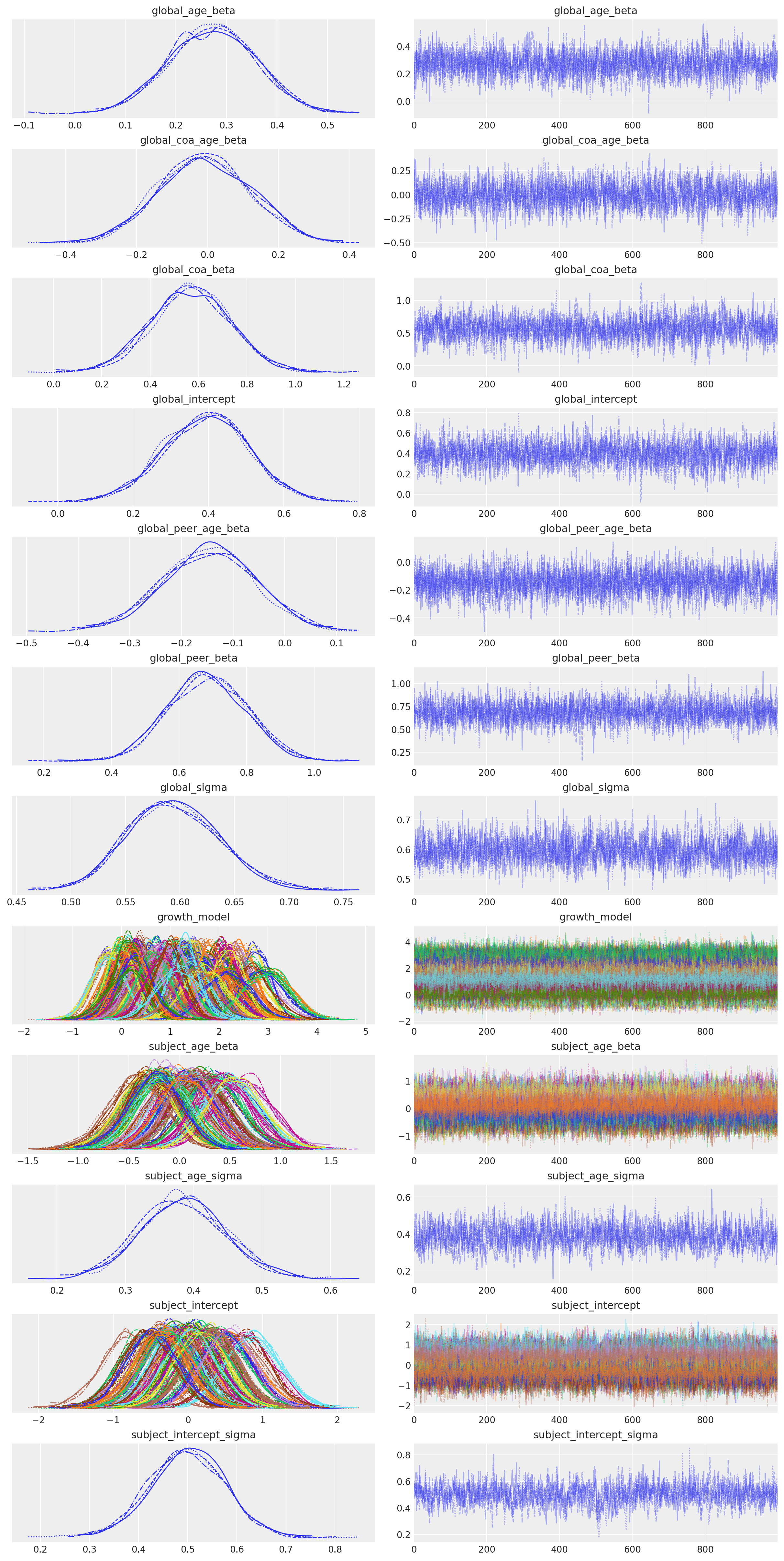
az.plot_trace(idata_m3);
az.summary(
    idata_m3,
    var_names=[
        "global_intercept",
        "global_sigma",
        "global_age_beta",
        "global_coa_age_beta",
        "global_peer_beta",
        "global_peer_age_beta",
        "subject_intercept_sigma",
        "subject_age_sigma",
    ],
)
| mean | sd | hdi_3% | hdi_97% | mcse_mean | mcse_sd | ess_bulk | ess_tail | r_hat | |
|---|---|---|---|---|---|---|---|---|---|
| global_intercept | 0.395 | 0.112 | 0.177 | 0.601 | 0.002 | 0.002 | 2210.0 | 2599.0 | 1.0 |
| global_sigma | 0.595 | 0.042 | 0.522 | 0.676 | 0.001 | 0.001 | 1589.0 | 2884.0 | 1.0 |
| global_age_beta | 0.273 | 0.085 | 0.117 | 0.434 | 0.002 | 0.001 | 2382.0 | 2805.0 | 1.0 |
| global_coa_age_beta | -0.007 | 0.128 | -0.245 | 0.225 | 0.003 | 0.002 | 2364.0 | 2734.0 | 1.0 |
| global_peer_beta | 0.683 | 0.114 | 0.483 | 0.904 | 0.002 | 0.001 | 3072.0 | 2872.0 | 1.0 |
| global_peer_age_beta | -0.146 | 0.090 | -0.313 | 0.022 | 0.002 | 0.001 | 3080.0 | 2617.0 | 1.0 |
| subject_intercept_sigma | 0.500 | 0.077 | 0.356 | 0.647 | 0.002 | 0.002 | 1023.0 | 1231.0 | 1.0 |
| subject_age_sigma | 0.384 | 0.061 | 0.271 | 0.497 | 0.002 | 0.001 | 1080.0 | 1407.0 | 1.0 |
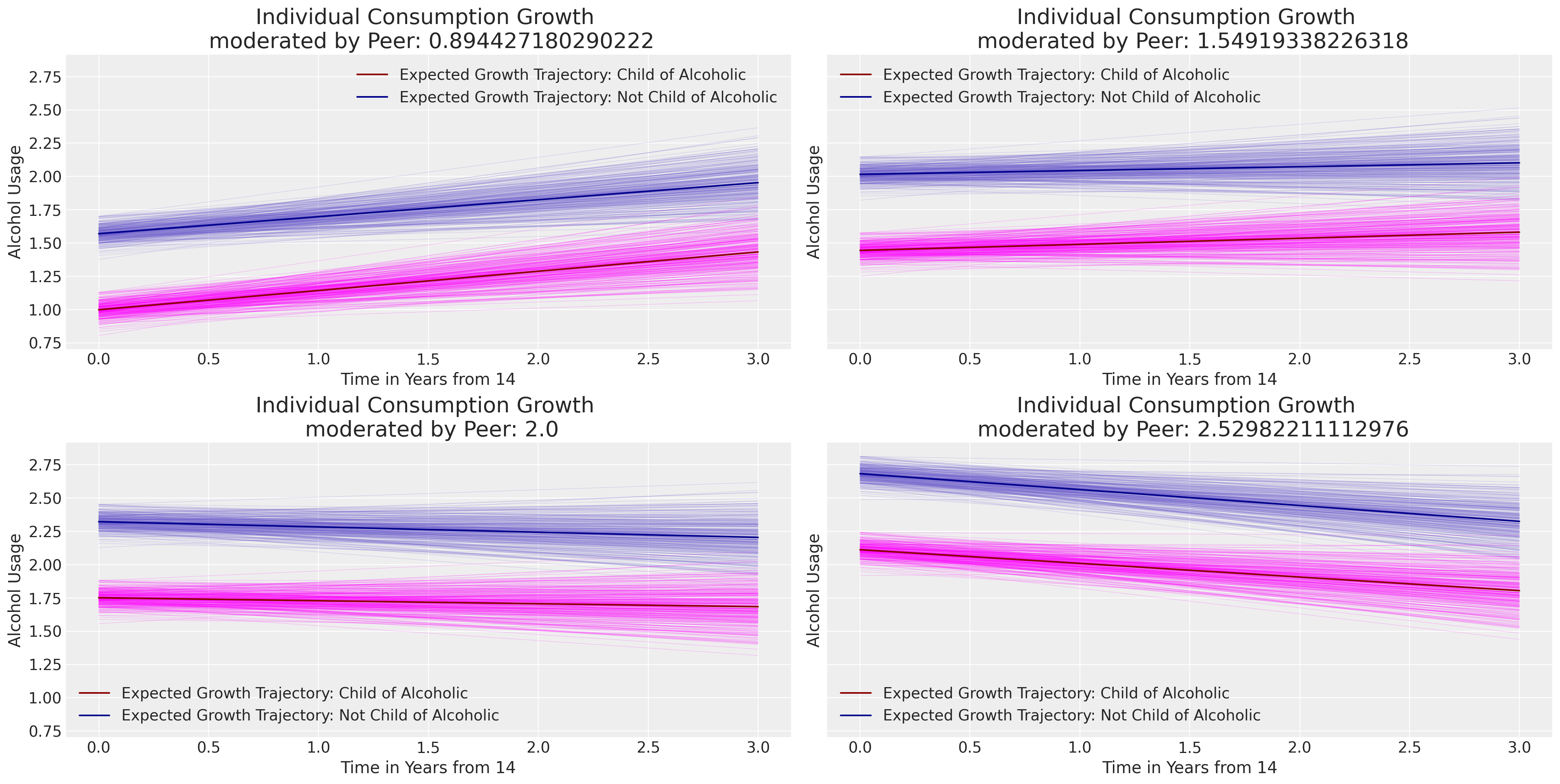
接下来,我们将绘制个体在父母和同伴关系条件下的典型变化轨迹。注意数据中的同伴评分如何推动多项式曲线的截距沿图表的y轴上升。
Show code cell source
fig, axs = plt.subplots(2, 2, figsize=(20, 10), sharey=True)
axs = axs.flatten()
posterior = az.extract(idata_m3.posterior, num_samples=300)
intercept_group_specific = posterior["subject_intercept"].mean(dim="ids")
slope_group_specific = posterior["subject_age_beta"].mean(dim="ids")
a = posterior["global_intercept"].mean() + intercept_group_specific
b = posterior["global_age_beta"].mean() + slope_group_specific
b_coa = posterior["global_coa_beta"].mean()
b_coa_age = posterior["global_coa_age_beta"].mean()
b_peer = posterior["global_peer_beta"].mean()
b_peer_age = posterior["global_peer_age_beta"].mean()

time_xi = xr.DataArray(np.arange(4))
for q, i in zip([0.5, 0.75, 0.90, 0.99], [0, 1, 2, 3]):
    q_v = df["peer"].quantile(q)
    f1 = (
        a
        + b * time_xi
        + b_coa * 1
        + b_coa_age * (time_xi * 1)
        + b_peer * q_v
        + b_peer_age * (time_xi * q_v)
    ).T
    f2 = (
        a
        + b * time_xi
        + b_coa * 0
        + b_coa_age * (time_xi * 0)
        + b_peer * q_v
        + b_peer_age * (time_xi * q_v)
    ).T
    axs[i].plot(time_xi, f1, color="slateblue", alpha=0.2, linewidth=0.5)
    axs[i].plot(time_xi, f2, color="magenta", alpha=0.2, linewidth=0.5)
    axs[i].plot(
        time_xi,
        f2.mean(axis=1),
        color="darkred",
        label="Expected Growth Trajectory: Child of Alcoholic",
    )
    axs[i].plot(
        time_xi,
        f1.mean(axis=1),
        color="darkblue",
        label="Expected Growth Trajectory: Not Child of Alcoholic",
    )
    axs[i].set_ylabel("Alcohol Usage")
    axs[i].set_xlabel("Time in Years from 14")
    axs[i].legend()
    axs[i].set_title(f"Individual Consumption Growth \n moderated by Peer: {q_v}", fontsize=20);
模型估计的比较#
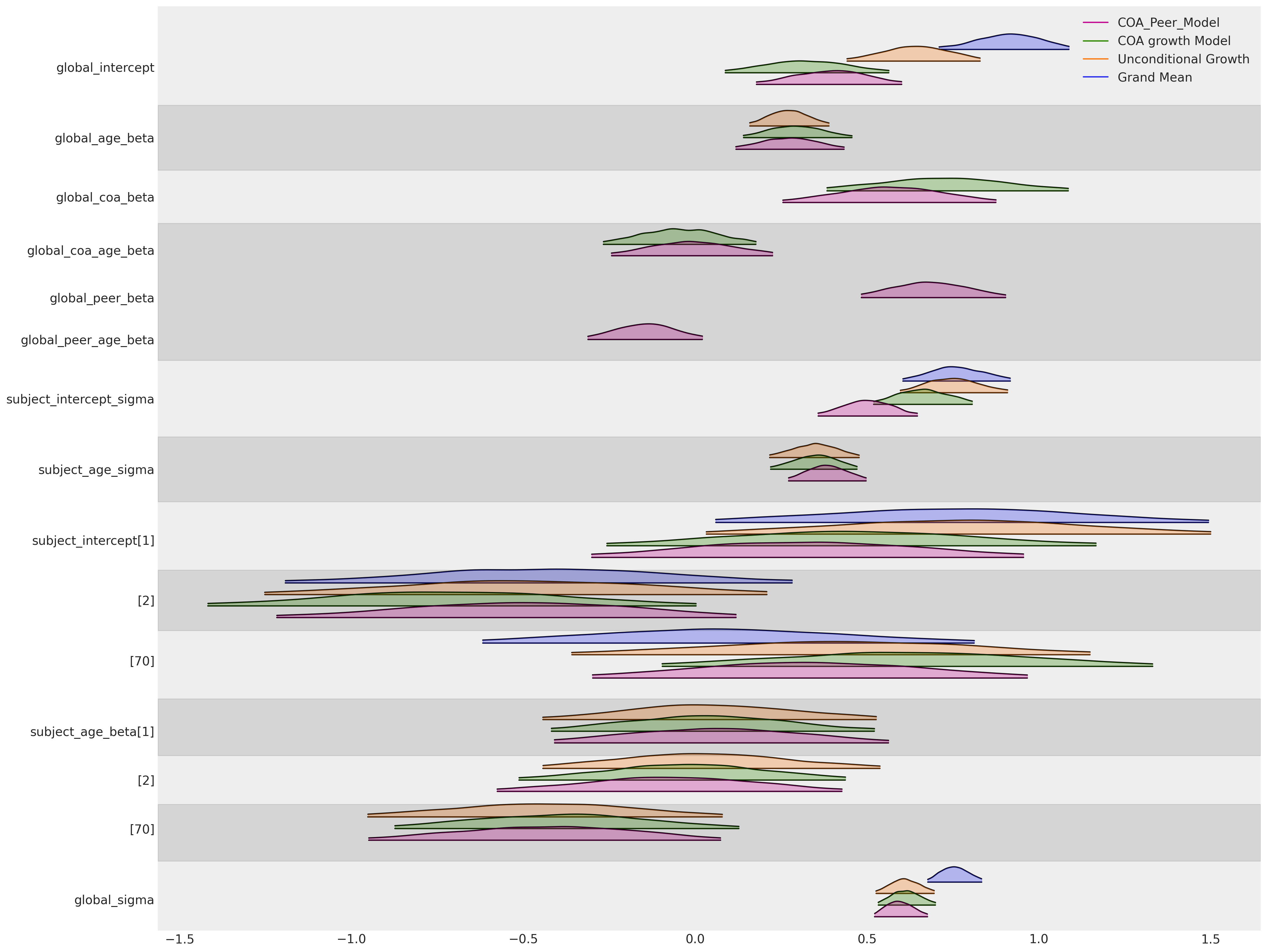
最后,综合我们迄今为止的所有建模工作,我们可以从上述图表中看到一些明显的现象:(i) 年龄项的全局斜率参数在所有三个包含它的模型中都非常稳定。同样,对于显示的三个个体中的每一个的特定主题斜率参数也是如此。全局截距参数被拉向零,因为我们可以将更多的结果效应抵消到父母和同伴关系的影响中。父母酗酒的全局效应在我们拟合的模型中大致一致。
然而,需要注意的是——解释这种层次模型的结果可能会很困难,特定参数的含义可能会根据模型性质和变量测量尺度而有所偏差。在本笔记本中,我们专注于理解由不同输入数据值引起的后验预测轨迹中的边际效应所隐含的对比。这通常是理解模型对所讨论增长轨迹所学内容的最清晰方式。
az.plot_forest(
    [idata_m0, idata_m1, idata_m2, idata_m3],
    model_names=["Grand Mean", "Unconditional Growth", "COA growth Model", "COA_Peer_Model"],
    var_names=[
        "global_intercept",
        "global_age_beta",
        "global_coa_beta",
        "global_coa_age_beta",
        "global_peer_beta",
        "global_peer_age_beta",
        "subject_intercept_sigma",
        "subject_age_sigma",
        "subject_intercept",
        "subject_age_beta",
        "global_sigma",
    ],
    figsize=(20, 15),
    kind="ridgeplot",
    combined=True,
    ridgeplot_alpha=0.3,
    coords={"ids": [1, 2, 70]},
);
对于模型的数值摘要,Willett 和 Singer 建议使用偏差统计量。在贝叶斯工作流程中,我们将使用 LOO。
compare = az.compare(
    {
        "Grand Mean": idata_m0,
        "Unconditional Growth": idata_m1,
        "COA growth Model": idata_m2,
        "COA_Peer_Model": idata_m3,
    },
)
compare
/home/osvaldo/proyectos/00_BM/arviz-devs/arviz/arviz/stats/stats.py:795: UserWarning: Estimated shape parameter of Pareto distribution is greater than 0.70 for one or more samples. You should consider using a more robust model, this is because importance sampling is less likely to work well if the marginal posterior and LOO posterior are very different. This is more likely to happen with a non-robust model and highly influential observations.
  warnings.warn(
| rank | elpd_loo | p_loo | elpd_diff | weight | se | dse | warning | scale | |
|---|---|---|---|---|---|---|---|---|---|
| COA_Peer_Model | 0 | -280.547108 | 88.317101 | 0.000000 | 0.919592 | 12.286282 | 0.000000 | True | log |
| COA growth Model | 1 | -289.267096 | 89.708607 | 8.719988 | 0.000000 | 12.723690 | 4.226971 | True | log |
| Unconditional Growth | 2 | -289.776375 | 91.650347 | 9.229267 | 0.080408 | 12.808780 | 4.784305 | True | log |
| Grand Mean | 3 | -315.943445 | 58.611975 | 35.396337 | 0.000000 | 12.426100 | 8.431326 | True | log |
az.plot_compare(compare, figsize=(10, 4));
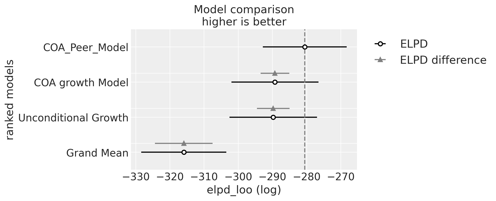
Willett 和 Singer 详细讨论了如何分析模型之间的差异,并评估不同的变异来源,以得出关于预测变量与结果之间关系的多个汇总统计数据。我们强烈推荐它作为对感兴趣读者的深入探讨。
插曲:使用Bambi的分层模型#
虽然我们直接在 PyMC 中拟合这些模型,但还有一个替代的贝叶斯多层次建模包 Bambi,它是基于 PyMC 框架构建的。Bambi 在多个方面进行了优化,以适应分层贝叶斯模型,包括使用公式指定模型结构的选项。我们将简要演示如何使用这种语法拟合最后一个模型。
公式规范使用 1 表示截距项,并使用条件 | 运算符表示主题级别参数与上述方式指定的相同类型的全局参数的组合。我们将添加截距项和焦点变量年龄的beta系数的主体特定修改,如上述模型所示。我们使用 Bambi 公式语法中的语法 (1 + age_14 | id) 来实现这一点。
formula = "alcuse ~ 1 + age_14 + coa + cpeer + age_14:coa + age_14:cpeer + (1 + age_14 | id)"
model = bmb.Model(formula, df)

# Fit the model using 1000 on each of 4 chains
idata_bambi = model.fit(draws=1000, chains=4)
model.predict(idata_bambi, kind="pps")
idata_bambi
Auto-assigning NUTS sampler...
Initializing NUTS using jitter+adapt_diag...
Multiprocess sampling (4 chains in 4 jobs)
NUTS: [sigma, Intercept, age_14, coa, cpeer, age_14:coa, age_14:cpeer, 1|id_sigma, 1|id_offset, age_14|id_sigma, age_14|id_offset]
Sampling 4 chains for 1_000 tune and 1_000 draw iterations (4_000 + 4_000 draws total) took 12 seconds.
/home/osvaldo/anaconda3/envs/pymc/lib/python3.11/site-packages/bambi/models.py:858: FutureWarning: 'pps' has been replaced by 'response' and is not going to work in the future
  warnings.warn(
-
<xarray.Dataset> Dimensions: (chain: 4, draw: 1000, id__factor_dim: 82, __obs__: 246) Coordinates: * chain (chain) int64 0 1 2 3 * draw (draw) int64 0 1 2 3 4 5 6 ... 993 994 995 996 997 998 999 * id__factor_dim (id__factor_dim) <U2 '1' '2' '3' '4' ... '80' '81' '82' * __obs__ (__obs__) int64 0 1 2 3 4 5 6 ... 240 241 242 243 244 245 Data variables: 1|id (chain, draw, id__factor_dim) float64 0.5433 ... -0.2393 1|id_sigma (chain, draw) float64 0.4957 0.577 0.5026 ... 0.4642 0.4398 Intercept (chain, draw) float64 0.4438 0.3648 ... 0.4879 0.3531 age_14 (chain, draw) float64 0.3028 0.3717 ... 0.2674 0.1804 age_14:coa (chain, draw) float64 0.0516 -0.03368 ... 0.04597 0.1363 age_14:cpeer (chain, draw) float64 -0.1768 -0.1898 ... -0.1679 -0.1466 age_14|id (chain, draw, id__factor_dim) float64 -0.05741 ... 0.04858 age_14|id_sigma (chain, draw) float64 0.4117 0.3575 ... 0.4522 0.3759 coa (chain, draw) float64 0.674 0.7293 0.6766 ... 0.5017 0.6076 cpeer (chain, draw) float64 0.8057 0.8209 ... 0.6051 0.6673 sigma (chain, draw) float64 0.5183 0.6357 ... 0.5916 0.6073 mu (chain, draw, __obs__) float64 1.86 2.113 ... 0.9535 1.011 Attributes: created_at: 2024-08-17T17:08:19.195670+00:00 arviz_version: 0.20.0.dev0 inference_library: pymc inference_library_version: 5.16.2+20.g747fda319 sampling_time: 11.552397727966309 tuning_steps: 1000 modeling_interface: bambi modeling_interface_version: 0.14.0 -
<xarray.Dataset> Dimensions: (chain: 4, draw: 1000, __obs__: 246) Coordinates: * chain (chain) int64 0 1 2 3 * draw (draw) int64 0 1 2 3 4 5 6 7 8 ... 992 993 994 995 996 997 998 999 * __obs__ (__obs__) int64 0 1 2 3 4 5 6 7 ... 238 239 240 241 242 243 244 245 Data variables: alcuse (chain, draw, __obs__) float64 1.217 2.066 2.677 ... 1.751 0.3636 Attributes: modeling_interface: bambi modeling_interface_version: 0.14.0 -
<xarray.Dataset> Dimensions: (chain: 4, draw: 1000) Coordinates: * chain (chain) int64 0 1 2 3 * draw (draw) int64 0 1 2 3 4 5 ... 994 995 996 997 998 999 Data variables: (12/17) acceptance_rate (chain, draw) float64 0.6227 0.6105 ... 0.9299 0.6517 diverging (chain, draw) bool False False False ... False False energy (chain, draw) float64 538.9 541.1 ... 553.3 541.8 energy_error (chain, draw) float64 0.4803 0.632 ... -0.7672 0.3856 index_in_trajectory (chain, draw) int64 -15 6 -6 -8 -7 10 ... 8 7 6 -11 7 largest_eigval (chain, draw) float64 nan nan nan nan ... nan nan nan ... ... process_time_diff (chain, draw) float64 0.003959 0.004457 ... 0.003284 reached_max_treedepth (chain, draw) bool False False False ... False False smallest_eigval (chain, draw) float64 nan nan nan nan ... nan nan nan step_size (chain, draw) float64 0.3006 0.3006 ... 0.286 0.286 step_size_bar (chain, draw) float64 0.2747 0.2747 ... 0.2719 0.2719 tree_depth (chain, draw) int64 4 4 4 4 4 4 4 4 ... 4 4 4 4 4 4 4 Attributes: created_at: 2024-08-17T17:08:19.205959+00:00 arviz_version: 0.20.0.dev0 inference_library: pymc inference_library_version: 5.16.2+20.g747fda319 sampling_time: 11.552397727966309 tuning_steps: 1000 modeling_interface: bambi modeling_interface_version: 0.14.0 -
<xarray.Dataset>
Dimensions:  (__obs__: 246)
Coordinates:
  * __obs__  (__obs__) int64 0 1 2 3 4 5 6 7 ... 238 239 240 241 242 243 244 245
Data variables:
    alcuse   (__obs__) float64 1.732 2.0 2.0 0.0 0.0 ... 0.0 0.0 0.0 1.414 1.0
Attributes:
    created_at:                  2024-08-17T17:08:19.209059+00:00
    arviz_version:               0.20.0.dev0
    inference_library:           pymc
    inference_library_version:   5.16.2+20.g747fda319
    modeling_interface:          bambi
    modeling_interface_version:  0.14.0
模型定义得很好,详细说明了层次结构和主题级别的参数结构。默认情况下,Bambi 模型会分配先验并使用非中心参数化。Bambi 模型定义使用了常见和组级别效应的语言,而不是我们在此示例中一直使用的全局和主题的区别。再次强调,重要的是层次结构,而不是名称。
model
       Formula: alcuse ~ 1 + age_14 + coa + cpeer + age_14:coa + age_14:cpeer + (1 + age_14 | id)
        Family: gaussian
          Link: mu = identity
  Observations: 246
        Priors:
    target = mu
        Common-level effects
            Intercept ~ Normal(mu: 0.922, sigma: 5.0974)
            age_14 ~ Normal(mu: 0.0, sigma: 3.2485)
            coa ~ Normal(mu: 0.0, sigma: 5.3302)
            cpeer ~ Normal(mu: 0.0, sigma: 3.6587)
            age_14:coa ~ Normal(mu: 0.0, sigma: 3.5816)
            age_14:cpeer ~ Normal(mu: 0.0, sigma: 2.834)

        Group-level effects
            1|id ~ Normal(mu: 0.0, sigma: HalfNormal(sigma: 5.0974))
            age_14|id ~ Normal(mu: 0.0, sigma: HalfNormal(sigma: 3.2485))

        Auxiliary parameters
            sigma ~ HalfStudentT(nu: 4.0, sigma: 1.0609)
------
* To see a plot of the priors call the .plot_priors() method.
* To see a summary or plot of the posterior pass the object returned by .fit() to az.summary() or az.plot_trace()
由于使用了偏移量来实现非中心参数化,模型图看起来也有所不同。
model.graph()

az.summary(
    idata_bambi,
    var_names=[
        "Intercept",
        "age_14",
        "coa",
        "cpeer",
        "age_14:coa",
        "age_14:cpeer",
        "1|id_sigma",
        "age_14|id_sigma",
        "sigma",
    ],
)
| mean | sd | hdi_3% | hdi_97% | mcse_mean | mcse_sd | ess_bulk | ess_tail | r_hat | |
|---|---|---|---|---|---|---|---|---|---|
| Intercept | 0.390 | 0.107 | 0.170 | 0.579 | 0.002 | 0.001 | 2855.0 | 3083.0 | 1.0 |
| age_14 | 0.277 | 0.084 | 0.123 | 0.438 | 0.002 | 0.001 | 2283.0 | 2994.0 | 1.0 |
| coa | 0.581 | 0.162 | 0.268 | 0.873 | 0.003 | 0.002 | 2784.0 | 3038.0 | 1.0 |
| cpeer | 0.692 | 0.116 | 0.480 | 0.914 | 0.002 | 0.002 | 2959.0 | 3040.0 | 1.0 |
| age_14:coa | -0.013 | 0.123 | -0.237 | 0.219 | 0.002 | 0.002 | 2441.0 | 2928.0 | 1.0 |
| age_14:cpeer | -0.150 | 0.087 | -0.303 | 0.020 | 0.002 | 0.001 | 2890.0 | 3103.0 | 1.0 |
| 1|id_sigma | 0.502 | 0.078 | 0.356 | 0.645 | 0.002 | 0.002 | 1315.0 | 2130.0 | 1.0 |
| age_14|id_sigma | 0.379 | 0.060 | 0.262 | 0.488 | 0.002 | 0.001 | 1244.0 | 1860.0 | 1.0 |
| sigma | 0.595 | 0.043 | 0.516 | 0.674 | 0.001 | 0.001 | 1124.0 | 2355.0 | 1.0 |
az.plot_forest(
    idata_bambi,
    var_names=[
        "Intercept",
        "age_14",
        "coa",
        "cpeer",
        "age_14:coa",
        "age_14:cpeer",
        "1|id_sigma",
        "age_14|id_sigma",
        "sigma",
    ],
    figsize=(20, 6),
    kind="ridgeplot",
    combined=True,
    ridgeplot_alpha=0.3,
);
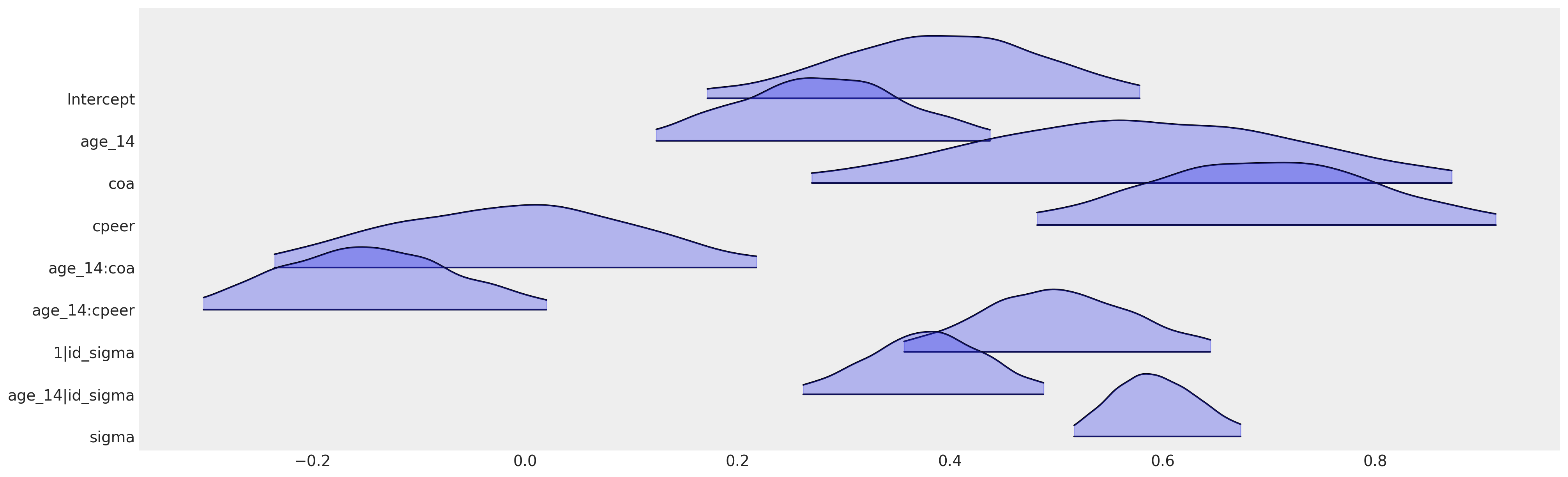
我们可以在这里看到,bambi模型规范如何恢复了与使用PyMC推导出的相同的参数化。在实际应用和生产环境中,如果您使用的是贝叶斯分层模型,您应该尽可能使用bambi。它在许多用例中都很灵活,您可能只需要在高度定制的模型中使用PyMC,因为在这些模型中,模型规范的灵活性无法通过公式语法的约束来满足。
非线性变化轨迹#
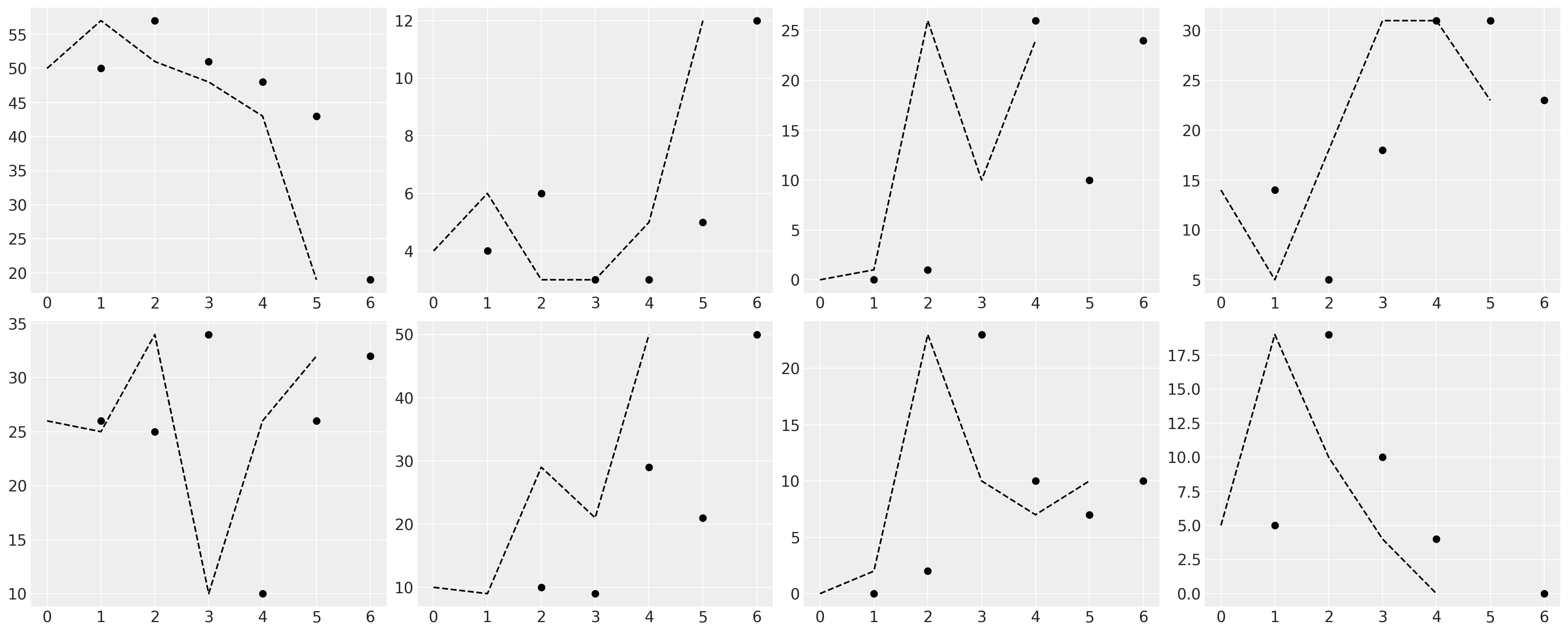
接下来我们将研究一个数据集,其中个体的轨迹显示出个体间行为的剧烈波动。该数据报告了每个儿童的外化行为得分。这可以衡量多种行为,包括但不限于:身体攻击、言语欺凌、关系攻击、反抗、盗窃和破坏行为。得分越高,儿童表现出的外化行为越多。该量表的下限为0,最高可能得分为68。每个儿童在学校的每个年级都会被测量这些行为。
try:
    df_external = pd.read_csv("../data/external_pp.csv")
except FileNotFoundError:
    df_external = pd.read_csv(pm.get_data("external_pp.csv"))

df_external.head()
| ID | EXTERNAL | FEMALE | TIME | GRADE | |
|---|---|---|---|---|---|
| 0 | 1 | 50 | 0 | 0 | 1 |
| 1 | 1 | 57 | 0 | 1 | 2 |
| 2 | 1 | 51 | 0 | 2 | 3 |
| 3 | 1 | 48 | 0 | 3 | 4 |
| 4 | 1 | 43 | 0 | 4 | 5 |
fig, axs = plt.subplots(2, 4, figsize=(20, 8))
axs = axs.flatten()
for ax, id in zip(axs, range(9)[1:9]):
    temp = df_external[df_external["ID"] == id]
    ax.plot(temp["GRADE"], temp["EXTERNAL"], "o", color="black")
    z = lowess(temp["EXTERNAL"], temp["GRADE"], 1 / 2)
    ax.plot(z[:, 1], "--", color="black")
fig, axs = plt.subplots(2, 3, figsize=(20, 6))
axs = axs.flatten()
for ax, g in zip(axs, [1, 2, 3, 4, 5, 6]):
    temp = df_external[df_external["GRADE"] == g]
    ax.hist(temp["EXTERNAL"], bins=10, ec="black", color="C0")
    ax.set_title(f"External Behaviour in Grade {g}")
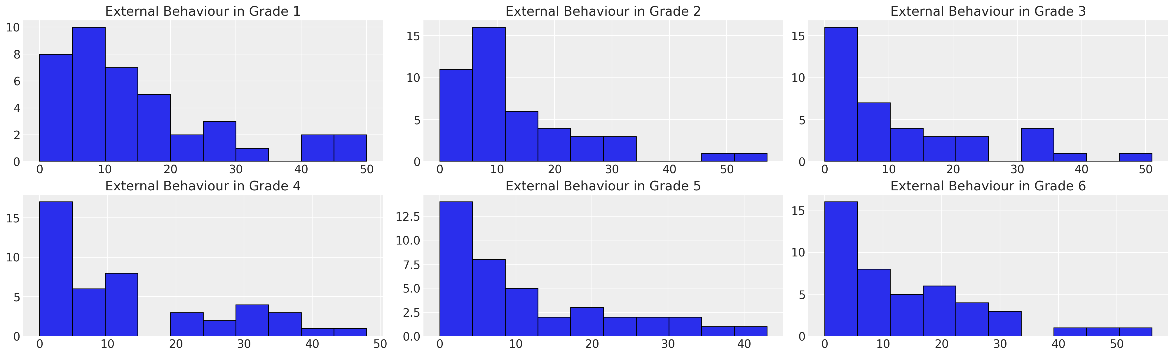
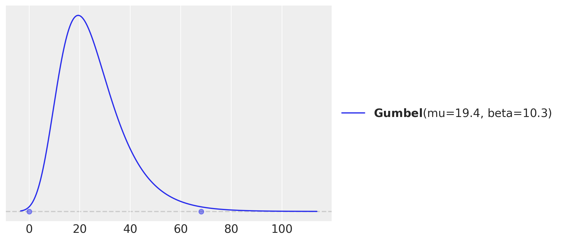
我们可以看到,数据集中存在一个强烈的偏斜,趋向于低external分数。我们将在这里偏离Willett和Singer的演示,尝试将这个分布建模为一个带有删失的Gumbel分布。为此,我们将让PyMC找到一个在Gumbel分布上合理的先验。
pz.maxent(pz.Gumbel(), lower=0, upper=68, mass=0.99);
一个最小模型#
与之前一样,我们将从一个相当简单的模型开始,指定一个层次模型,其中每个个体修改总体均值。我们允许使用非正态的截断似然项。
id_indx, unique_ids = pd.factorize(df_external["ID"])
coords = {"ids": unique_ids, "obs": range(len(df_external["EXTERNAL"]))}
with pm.Model(coords=coords) as model:
    external = pm.MutableData("external_data", df_external["EXTERNAL"].values + 1e-25)
    global_intercept = pm.Normal("global_intercept", 6, 1)
    global_sigma = pm.HalfNormal("global_sigma", 7)

    subject_intercept_sigma = pm.HalfNormal("subject_intercept_sigma", 5)
    subject_intercept = pm.Normal("subject_intercept", 0, subject_intercept_sigma, dims="ids")
    mu = pm.Deterministic("mu", global_intercept + subject_intercept[id_indx])
    outcome_latent = pm.Gumbel.dist(mu, global_sigma)
    outcome = pm.Censored(
        "outcome", outcome_latent, lower=0, upper=68, observed=external, dims="obs"
    )
    idata_m4 = pm.sample_prior_predictive()
    idata_m4.extend(
        pm.sample(random_seed=100, target_accept=0.95, idata_kwargs={"log_likelihood": True})
    )
    idata_m4.extend(pm.sample_posterior_predictive(idata_m4))

pm.model_to_graphviz(model)
/home/osvaldo/proyectos/00_BM/pymc-devs/pymc/pymc/data.py:304: FutureWarning: MutableData is deprecated. All Data variables are now mutable. Use Data instead.
  warnings.warn(
Sampling: [global_intercept, global_sigma, outcome, subject_intercept, subject_intercept_sigma]
Auto-assigning NUTS sampler...
Initializing NUTS using jitter+adapt_diag...
Multiprocess sampling (4 chains in 4 jobs)
NUTS: [global_intercept, global_sigma, subject_intercept_sigma, subject_intercept]
Sampling 4 chains for 1_000 tune and 1_000 draw iterations (4_000 + 4_000 draws total) took 11 seconds.
Sampling: [outcome]

az.summary(idata_m4, var_names=["global_intercept", "global_sigma", "subject_intercept_sigma"])
| mean | sd | hdi_3% | hdi_97% | mcse_mean | mcse_sd | ess_bulk | ess_tail | r_hat | |
|---|---|---|---|---|---|---|---|---|---|
| global_intercept | 7.347 | 0.754 | 5.950 | 8.769 | 0.019 | 0.013 | 1612.0 | 2336.0 | 1.0 |
| global_sigma | 6.810 | 0.380 | 6.118 | 7.546 | 0.006 | 0.004 | 4726.0 | 2892.0 | 1.0 |
| subject_intercept_sigma | 6.802 | 0.895 | 5.158 | 8.459 | 0.016 | 0.011 | 3045.0 | 2681.0 | 1.0 |
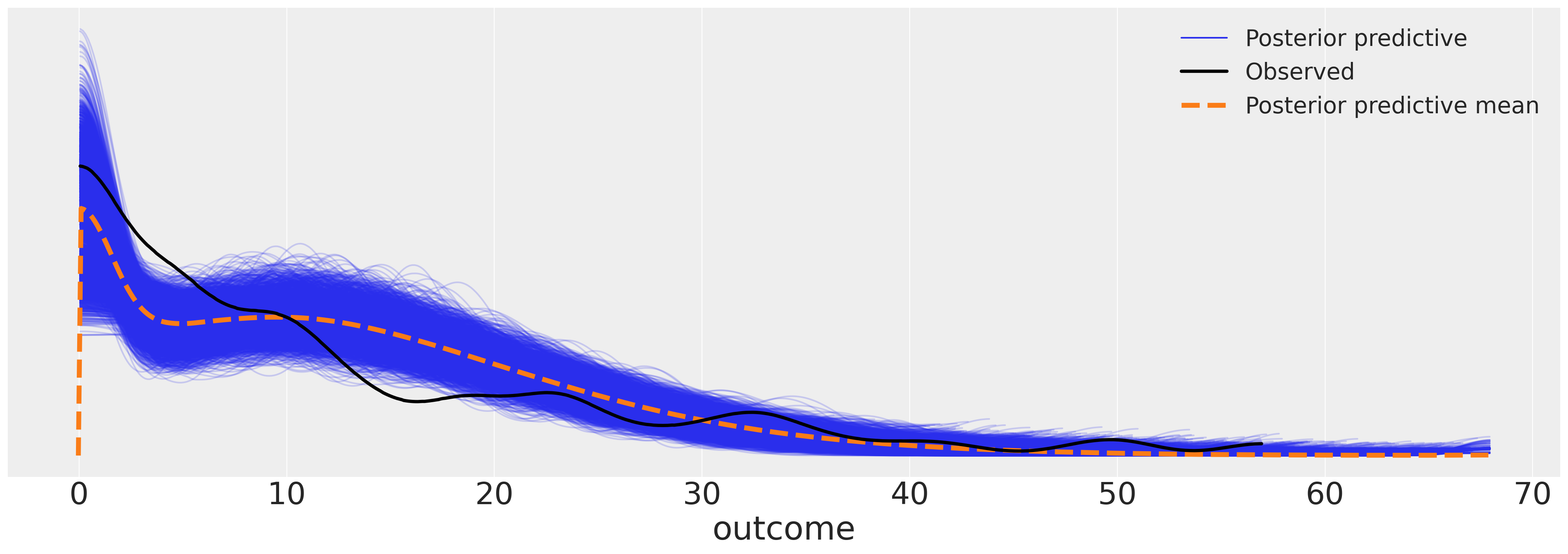
az.plot_ppc(idata_m4, figsize=(20, 7))
<Axes: xlabel='outcome'>

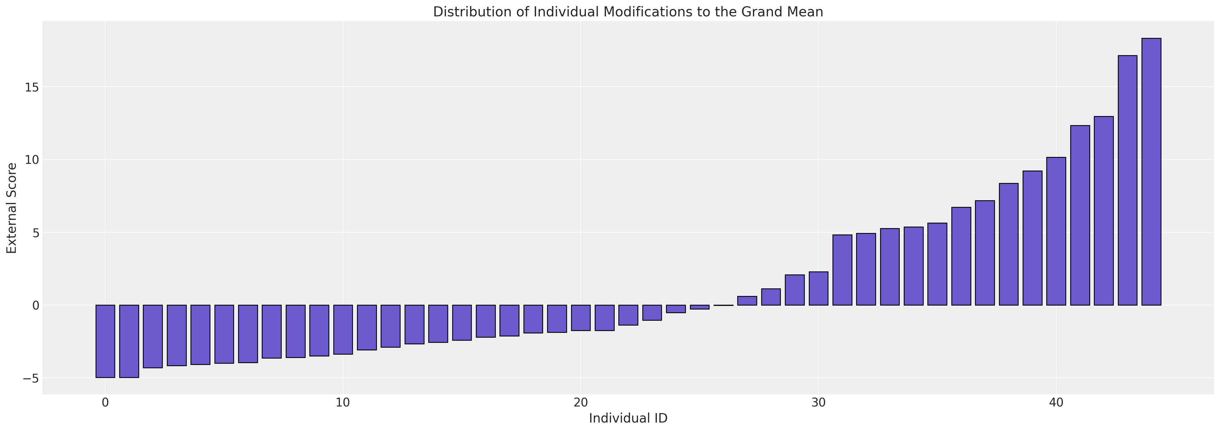
fig, ax = plt.subplots(figsize=(20, 7))
expected_individual_mean = idata_m4.posterior["subject_intercept"].mean(axis=1).values[0]

ax.bar(
    range(len(expected_individual_mean)),
    np.sort(expected_individual_mean),
    color="slateblue",
    ec="black",
)
ax.set_xlabel("Individual ID")
ax.set_ylabel("External Score")
ax.set_title("Distribution of Individual Modifications to the Grand Mean");
随时间变化的行为#
我们现在以分层的方式对行为随时间的演变进行建模。我们从一个简单的分层线性回归开始,以年级作为焦点预测因子。
id_indx, unique_ids = pd.factorize(df_external["ID"])
coords = {"ids": unique_ids, "obs": range(len(df_external["EXTERNAL"]))}
with pm.Model(coords=coords) as model:
    grade = pm.MutableData("grade_data", df_external["GRADE"].values)
    external = pm.MutableData("external_data", df_external["EXTERNAL"].values + 1e-25)
    global_intercept = pm.Normal("global_intercept", 6, 1)
    global_sigma = pm.Normal("global_sigma", 7, 0.5)
    global_beta_grade = pm.Normal("global_beta_grade", 0, 1)

    subject_intercept_sigma = pm.HalfNormal("subject_intercept_sigma", 2)
    subject_intercept = pm.Normal("subject_intercept", 5, subject_intercept_sigma, dims="ids")

    subject_beta_grade_sigma = pm.HalfNormal("subject_beta_grade_sigma", 1)
    subject_beta_grade = pm.Normal("subject_beta_grade", 0, subject_beta_grade_sigma, dims="ids")
    mu = pm.Deterministic(
        "mu",
        global_intercept
        + subject_intercept[id_indx]
        + (global_beta_grade + subject_beta_grade[id_indx]) * grade,
    )
    outcome_latent = pm.Gumbel.dist(mu, global_sigma)
    outcome = pm.Censored(
        "outcome", outcome_latent, lower=0, upper=68, observed=external, dims="obs"
    )
    idata_m5 = pm.sample_prior_predictive()
    idata_m5.extend(
        pm.sample(random_seed=100, target_accept=0.95, idata_kwargs={"log_likelihood": True})
    )
    idata_m5.extend(pm.sample_posterior_predictive(idata_m5))

pm.model_to_graphviz(model)
/home/osvaldo/proyectos/00_BM/pymc-devs/pymc/pymc/data.py:304: FutureWarning: MutableData is deprecated. All Data variables are now mutable. Use Data instead.
  warnings.warn(
Sampling: [global_beta_grade, global_intercept, global_sigma, outcome, subject_beta_grade, subject_beta_grade_sigma, subject_intercept, subject_intercept_sigma]
Auto-assigning NUTS sampler...
Initializing NUTS using jitter+adapt_diag...
Multiprocess sampling (4 chains in 4 jobs)
NUTS: [global_intercept, global_sigma, global_beta_grade, subject_intercept_sigma, subject_intercept, subject_beta_grade_sigma, subject_beta_grade]
Sampling 4 chains for 1_000 tune and 1_000 draw iterations (4_000 + 4_000 draws total) took 33 seconds.
There were 60 divergences after tuning. Increase `target_accept` or reparameterize.
The rhat statistic is larger than 1.01 for some parameters. This indicates problems during sampling. See https://arxiv.org/abs/1903.08008 for details
The effective sample size per chain is smaller than 100 for some parameters.  A higher number is needed for reliable rhat and ess computation. See https://arxiv.org/abs/1903.08008 for details
Sampling: [outcome]

az.summary(
    idata_m5,
    var_names=[
        "global_intercept",
        "global_sigma",
        "global_beta_grade",
        "subject_intercept_sigma",
        "subject_beta_grade_sigma",
    ],
)
| mean | sd | hdi_3% | hdi_97% | mcse_mean | mcse_sd | ess_bulk | ess_tail | r_hat | |
|---|---|---|---|---|---|---|---|---|---|
| global_intercept | 5.246 | 0.746 | 3.952 | 6.829 | 0.078 | 0.061 | 143.0 | 2169.0 | 1.09 |
| global_sigma | 6.875 | 0.279 | 6.343 | 7.456 | 0.004 | 0.003 | 3986.0 | 1885.0 | 1.39 |
| global_beta_grade | -0.262 | 0.242 | -0.673 | 0.253 | 0.028 | 0.020 | 99.0 | 1903.0 | 1.07 |
| subject_intercept_sigma | 5.320 | 0.887 | 3.416 | 6.789 | 0.133 | 0.095 | 55.0 | 976.0 | 1.06 |
| subject_beta_grade_sigma | 0.625 | 0.444 | 0.019 | 1.266 | 0.166 | 0.123 | 8.0 | 5.0 | 1.49 |
我们现在可以检查模型的后验预测图。结果似乎对数据拟合得相当合理。
az.plot_ppc(idata_m5, figsize=(20, 7));
但我们希望看到每个人的个体模型拟合情况。这里我们绘制了预期的轨迹。
Show code cell source
fig, ax = plt.subplots(figsize=(20, 7))
posterior = az.extract(idata_m5.posterior)
intercept_group_specific = posterior["subject_intercept"].mean("sample")
slope_group_specific = posterior["subject_beta_grade"].mean("sample")
a = posterior["global_intercept"].mean() + intercept_group_specific
b = posterior["global_beta_grade"].mean() + slope_group_specific

time_xi = xr.DataArray(np.arange(6))
ax.plot(time_xi, (a + b * time_xi).T, color="slateblue", alpha=0.6)
ax.plot(
    time_xi, (a.mean() + b.mean() * time_xi), color="red", lw=2, label="Expected Growth Trajectory"
)
ax.set_ylabel("Externalised Behaviour Score")
ax.set_xlabel("Time in Grade")
ax.legend()
ax.set_title("Within Individual Typical Trajctories", fontsize=20);
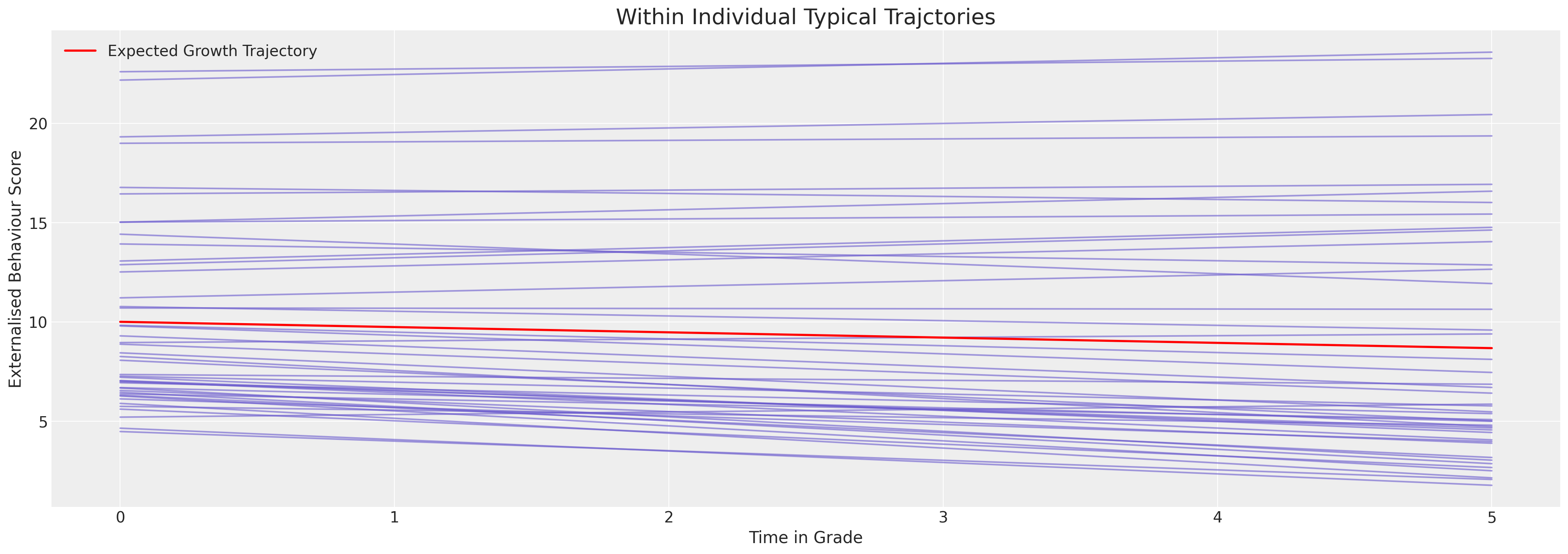
我们可以看到这里模型是如何被限制以非常线性的方式拟合行为轨迹的。第一印象是每个个体的行为模式相对稳定。但这实际上是模型无法表达行为数据曲率的结果。尽管如此,我们可以看到个体差异使得截距项在5到25的范围内变化。
多项式时间内的加法#
为了使模型更具灵活性以模拟随时间的变化,我们可以加入多项式项。
id_indx, unique_ids = pd.factorize(df_external["ID"])
coords = {"ids": unique_ids, "obs": range(len(df_external["EXTERNAL"]))}
with pm.Model(coords=coords) as model:
    grade = pm.MutableData("grade_data", df_external["GRADE"].values)
    grade2 = pm.MutableData("grade2_data", df_external["GRADE"].values ** 2)
    external = pm.MutableData("external_data", df_external["EXTERNAL"].values + 1e-25)

    global_intercept = pm.Normal("global_intercept", 6, 2)
    global_sigma = pm.Normal("global_sigma", 7, 1)
    global_beta_grade = pm.Normal("global_beta_grade", 0, 1)
    global_beta_grade2 = pm.Normal("global_beta_grade2", 0, 1)

    subject_intercept_sigma = pm.HalfNormal("subject_intercept_sigma", 1)
    subject_intercept = pm.Normal("subject_intercept", 2, subject_intercept_sigma, dims="ids")

    subject_beta_grade_sigma = pm.HalfNormal("subject_beta_grade_sigma", 1)
    subject_beta_grade = pm.Normal("subject_beta_grade", 0, subject_beta_grade_sigma, dims="ids")

    subject_beta_grade2_sigma = pm.HalfNormal("subject_beta_grade2_sigma", 1)
    subject_beta_grade2 = pm.Normal("subject_beta_grade2", 0, subject_beta_grade2_sigma, dims="ids")

    mu = pm.Deterministic(
        "mu",
        global_intercept
        + subject_intercept[id_indx]
        + (global_beta_grade + subject_beta_grade[id_indx]) * grade
        + (global_beta_grade2 + subject_beta_grade2[id_indx]) * grade2,
    )
    outcome_latent = pm.Gumbel.dist(mu, global_sigma)
    outcome = pm.Censored(
        "outcome", outcome_latent, lower=0, upper=68, observed=external, dims="obs"
    )
    idata_m6 = pm.sample_prior_predictive()
    idata_m6.extend(
        pm.sample(random_seed=100, target_accept=0.95, idata_kwargs={"log_likelihood": True})
    )
    idata_m6.extend(pm.sample_posterior_predictive(idata_m6))

pm.model_to_graphviz(model)
/home/osvaldo/proyectos/00_BM/pymc-devs/pymc/pymc/data.py:304: FutureWarning: MutableData is deprecated. All Data variables are now mutable. Use Data instead.
  warnings.warn(
Sampling: [global_beta_grade, global_beta_grade2, global_intercept, global_sigma, outcome, subject_beta_grade, subject_beta_grade2, subject_beta_grade2_sigma, subject_beta_grade_sigma, subject_intercept, subject_intercept_sigma]
Auto-assigning NUTS sampler...
Initializing NUTS using jitter+adapt_diag...
Multiprocess sampling (4 chains in 4 jobs)
NUTS: [global_intercept, global_sigma, global_beta_grade, global_beta_grade2, subject_intercept_sigma, subject_intercept, subject_beta_grade_sigma, subject_beta_grade, subject_beta_grade2_sigma, subject_beta_grade2]
Sampling 4 chains for 1_000 tune and 1_000 draw iterations (4_000 + 4_000 draws total) took 79 seconds.
There were 849 divergences after tuning. Increase `target_accept` or reparameterize.
The rhat statistic is larger than 1.01 for some parameters. This indicates problems during sampling. See https://arxiv.org/abs/1903.08008 for details
The effective sample size per chain is smaller than 100 for some parameters.  A higher number is needed for reliable rhat and ess computation. See https://arxiv.org/abs/1903.08008 for details
Sampling: [outcome]

az.summary(
    idata_m6,
    var_names=[
        "global_intercept",
        "global_sigma",
        "global_beta_grade",
        "global_beta_grade2",
        "subject_intercept_sigma",
        "subject_beta_grade_sigma",
        "subject_beta_grade2_sigma",
    ],
)
| mean | sd | hdi_3% | hdi_97% | mcse_mean | mcse_sd | ess_bulk | ess_tail | r_hat | |
|---|---|---|---|---|---|---|---|---|---|
| global_intercept | 6.160 | 1.136 | 4.591 | 8.464 | 0.306 | 0.221 | 16.0 | 1359.0 | 1.17 |
| global_sigma | 6.978 | 0.333 | 6.329 | 7.650 | 0.013 | 0.010 | 809.0 | 1315.0 | 1.53 |
| global_beta_grade | -0.117 | 0.591 | -1.328 | 0.958 | 0.040 | 0.065 | 590.0 | 1156.0 | 1.53 |
| global_beta_grade2 | 0.071 | 0.093 | -0.118 | 0.246 | 0.006 | 0.004 | 445.0 | 1403.0 | 1.53 |
| subject_intercept_sigma | 1.174 | 1.173 | 0.010 | 3.273 | 0.424 | 0.312 | 6.0 | 4.0 | 1.79 |
| subject_beta_grade_sigma | 1.337 | 0.293 | 0.745 | 1.731 | 0.083 | 0.063 | 13.0 | 393.0 | 1.22 |
| subject_beta_grade2_sigma | 0.081 | 0.076 | 0.001 | 0.212 | 0.027 | 0.020 | 6.0 | 4.0 | 1.67 |
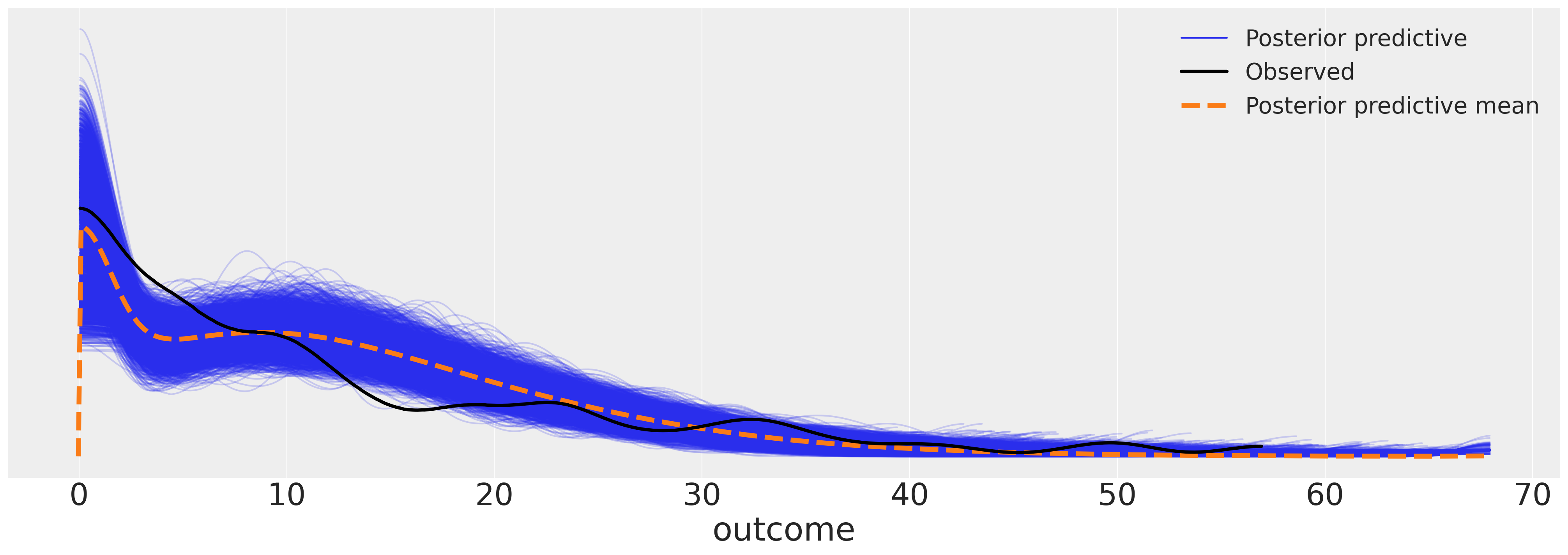
az.plot_ppc(idata_m6, figsize=(20, 7));
Show code cell source
fig, ax = plt.subplots(figsize=(20, 7))
posterior = az.extract(idata_m6.posterior)
intercept_group_specific = posterior["subject_intercept"].mean("sample")
slope_group_specific = posterior["subject_beta_grade"].mean("sample")
slope_group_specific_2 = posterior["subject_beta_grade2"].mean("sample")
a = posterior["global_intercept"].mean() + intercept_group_specific
b = posterior["global_beta_grade"].mean() + slope_group_specific
c = posterior["global_beta_grade2"].mean() + slope_group_specific_2

time_xi = xr.DataArray(np.arange(7))
ax.plot(time_xi, (a + b * time_xi + c * (time_xi**2)).T, color="slateblue", alpha=0.6)
ax.plot(
    time_xi,
    (a.mean() + b.mean() * time_xi + c.mean() * (time_xi**2)),
    color="red",
    lw=2,
    label="Expected Growth Trajectory",
)
ax.set_ylabel("Externalalising Behaviour Score")
ax.set_xlabel("Time in Grade")
ax.legend()
ax.set_title("Within Individual Typical Trajctories", fontsize=20);
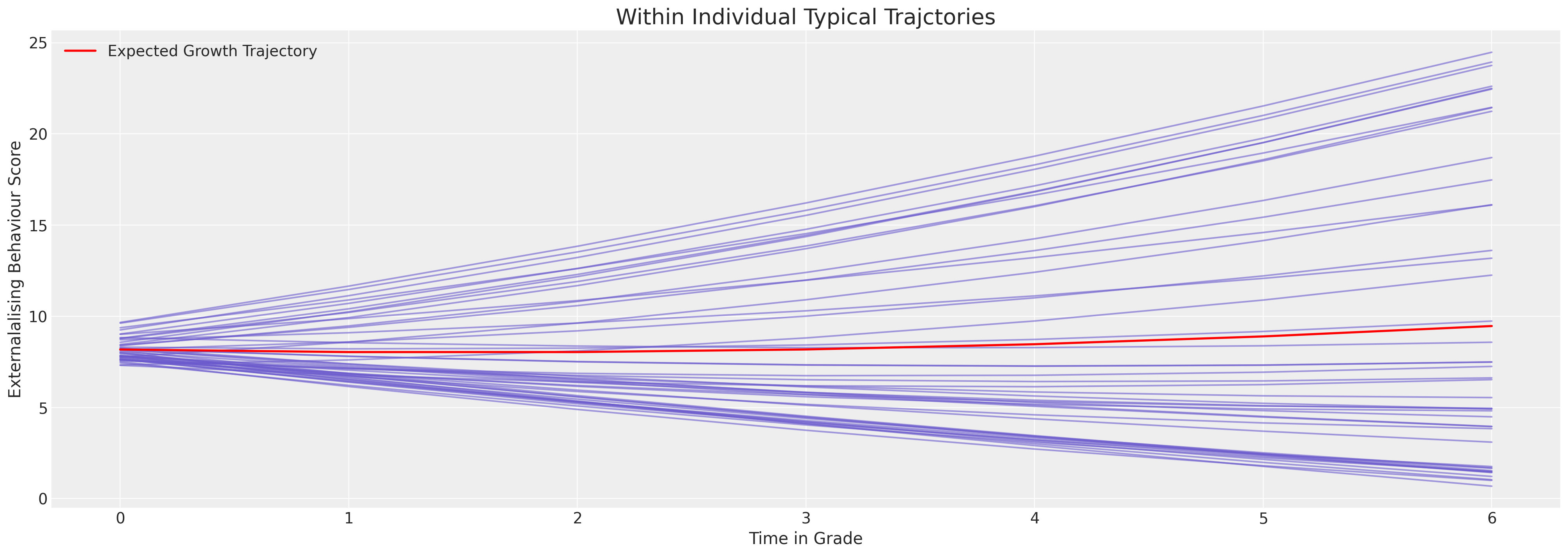
赋予模型更多的灵活性,使其能够描述更细致的增长轨迹。
按性别比较轨迹#
我们现在将允许模型更大的灵活性,并引入主体的性别来分析青少年的性别是否以及在多大程度上影响他们的行为变化。
id_indx, unique_ids = pd.factorize(df_external["ID"])
coords = {"ids": unique_ids, "obs": range(len(df_external["EXTERNAL"]))}
with pm.Model(coords=coords) as model:
    grade = pm.MutableData("grade_data", df_external["GRADE"].values)
    grade2 = pm.MutableData("grade2_data", df_external["GRADE"].values ** 2)
    grade3 = pm.MutableData("grade3_data", df_external["GRADE"].values ** 3)
    external = pm.MutableData("external_data", df_external["EXTERNAL"].values + 1e-25)
    female = pm.MutableData("female_data", df_external["FEMALE"].values)

    global_intercept = pm.Normal("global_intercept", 6, 2)
    global_sigma = pm.Normal("global_sigma", 7, 1)
    global_beta_grade = pm.Normal("global_beta_grade", 0, 1)
    global_beta_grade2 = pm.Normal("global_beta_grade2", 0, 1)
    global_beta_grade3 = pm.Normal("global_beta_grade3", 0, 1)
    global_beta_female = pm.Normal("global_beta_female", 0, 1)
    global_beta_female_grade = pm.Normal("global_beta_female_grade", 0, 1)
    global_beta_female_grade2 = pm.Normal("global_beta_female_grade2", 0, 1)
    global_beta_female_grade3 = pm.Normal("global_beta_female_grade3", 0, 1)

    subject_intercept_sigma = pm.Exponential("subject_intercept_sigma", 1)
    subject_intercept = pm.Normal("subject_intercept", 3, subject_intercept_sigma, dims="ids")

    subject_beta_grade_sigma = pm.Exponential("subject_beta_grade_sigma", 1)
    subject_beta_grade = pm.Normal("subject_beta_grade", 0, subject_beta_grade_sigma, dims="ids")

    subject_beta_grade2_sigma = pm.Exponential("subject_beta_grade2_sigma", 1)
    subject_beta_grade2 = pm.Normal("subject_beta_grade2", 0, subject_beta_grade2_sigma, dims="ids")

    subject_beta_grade3_sigma = pm.Exponential("subject_beta_grade3_sigma", 1)
    subject_beta_grade3 = pm.Normal("subject_beta_grade3", 0, subject_beta_grade3_sigma, dims="ids")

    mu = pm.Deterministic(
        "growth_model",
        global_intercept
        + subject_intercept[id_indx]
        + global_beta_female * female
        + global_beta_female_grade * (female * grade)
        + global_beta_female_grade2 * (female * grade2)
        + global_beta_female_grade3 * (female * grade3)
        + (global_beta_grade + subject_beta_grade[id_indx]) * grade
        + (global_beta_grade2 + subject_beta_grade2[id_indx]) * grade2
        + (global_beta_grade3 + subject_beta_grade3[id_indx]) * grade3,
    )

    outcome_latent = pm.Gumbel.dist(mu, global_sigma)
    outcome = pm.Censored(
        "outcome", outcome_latent, lower=0, upper=68, observed=external, dims="obs"
    )

    idata_m7 = pm.sample_prior_predictive()
    idata_m7.extend(
        pm.sample(
            draws=5000,
            random_seed=100,
            target_accept=0.99,
            nuts_sampler="numpyro",
            idata_kwargs={"log_likelihood": True},
        )
    )
    idata_m7.extend(pm.sample_posterior_predictive(idata_m7))
Show code cell output
/home/osvaldo/proyectos/00_BM/pymc-devs/pymc/pymc/data.py:304: FutureWarning: MutableData is deprecated. All Data variables are now mutable. Use Data instead.
  warnings.warn(
Sampling: [global_beta_female, global_beta_female_grade, global_beta_female_grade2, global_beta_female_grade3, global_beta_grade, global_beta_grade2, global_beta_grade3, global_intercept, global_sigma, outcome, subject_beta_grade, subject_beta_grade2, subject_beta_grade2_sigma, subject_beta_grade3, subject_beta_grade3_sigma, subject_beta_grade_sigma, subject_intercept, subject_intercept_sigma]
2024-08-17 14:12:54.209555: E external/xla/xla/service/slow_operation_alarm.cc:65] Constant folding an instruction is taking > 1s:

  %reduce.1 = f64[4,5000,254]{2,1,0} reduce(f64[4,5000,1,254]{3,2,1,0} %broadcast.80, f64[] %constant.25), dimensions={2}, to_apply=%region_2.83, metadata={op_name="jit(process_fn)/jit(main)/reduce_prod[axes=(2,)]" source_file="/tmp/tmp42m6glc9" source_line=43}

This isn't necessarily a bug; constant-folding is inherently a trade-off between compilation time and speed at runtime. XLA has some guards that attempt to keep constant folding from taking too long, but fundamentally you'll always be able to come up with an input program that takes a long time.

If you'd like to file a bug, run with envvar XLA_FLAGS=--xla_dump_to=/tmp/foo and attach the results.
2024-08-17 14:12:55.884724: E external/xla/xla/service/slow_operation_alarm.cc:133] The operation took 2.675309039s
Constant folding an instruction is taking > 1s:

  %reduce.1 = f64[4,5000,254]{2,1,0} reduce(f64[4,5000,1,254]{3,2,1,0} %broadcast.80, f64[] %constant.25), dimensions={2}, to_apply=%region_2.83, metadata={op_name="jit(process_fn)/jit(main)/reduce_prod[axes=(2,)]" source_file="/tmp/tmp42m6glc9" source_line=43}

This isn't necessarily a bug; constant-folding is inherently a trade-off between compilation time and speed at runtime. XLA has some guards that attempt to keep constant folding from taking too long, but fundamentally you'll always be able to come up with an input program that takes a long time.

If you'd like to file a bug, run with envvar XLA_FLAGS=--xla_dump_to=/tmp/foo and attach the results.
2024-08-17 14:12:57.889074: E external/xla/xla/service/slow_operation_alarm.cc:65] Constant folding an instruction is taking > 2s:

  %reduce.2 = f64[4,5000,254]{2,1,0} reduce(f64[4,5000,1,254]{3,2,1,0} %broadcast.81, f64[] %constant.25), dimensions={2}, to_apply=%region_2.83, metadata={op_name="jit(process_fn)/jit(main)/reduce_prod[axes=(2,)]" source_file="/tmp/tmp42m6glc9" source_line=43}

This isn't necessarily a bug; constant-folding is inherently a trade-off between compilation time and speed at runtime. XLA has some guards that attempt to keep constant folding from taking too long, but fundamentally you'll always be able to come up with an input program that takes a long time.

If you'd like to file a bug, run with envvar XLA_FLAGS=--xla_dump_to=/tmp/foo and attach the results.
2024-08-17 14:12:59.534352: E external/xla/xla/service/slow_operation_alarm.cc:133] The operation took 3.645368623s
Constant folding an instruction is taking > 2s:

  %reduce.2 = f64[4,5000,254]{2,1,0} reduce(f64[4,5000,1,254]{3,2,1,0} %broadcast.81, f64[] %constant.25), dimensions={2}, to_apply=%region_2.83, metadata={op_name="jit(process_fn)/jit(main)/reduce_prod[axes=(2,)]" source_file="/tmp/tmp42m6glc9" source_line=43}

This isn't necessarily a bug; constant-folding is inherently a trade-off between compilation time and speed at runtime. XLA has some guards that attempt to keep constant folding from taking too long, but fundamentally you'll always be able to come up with an input program that takes a long time.

If you'd like to file a bug, run with envvar XLA_FLAGS=--xla_dump_to=/tmp/foo and attach the results.
2024-08-17 14:13:33.840528: E external/xla/xla/service/slow_operation_alarm.cc:65] Constant folding an instruction is taking > 4s:

  %reduce.7 = f64[4,5000,254]{2,1,0} reduce(f64[4,5000,1,254]{3,2,1,0} %broadcast.65, f64[] %constant.28), dimensions={2}, to_apply=%region_0.68, metadata={op_name="jit(process_fn)/jit(main)/reduce_prod[axes=(2,)]" source_file="/tmp/tmppjx6pjej" source_line=37}

This isn't necessarily a bug; constant-folding is inherently a trade-off between compilation time and speed at runtime. XLA has some guards that attempt to keep constant folding from taking too long, but fundamentally you'll always be able to come up with an input program that takes a long time.

If you'd like to file a bug, run with envvar XLA_FLAGS=--xla_dump_to=/tmp/foo and attach the results.
2024-08-17 14:13:33.945988: E external/xla/xla/service/slow_operation_alarm.cc:133] The operation took 4.109097056s
Constant folding an instruction is taking > 4s:

  %reduce.7 = f64[4,5000,254]{2,1,0} reduce(f64[4,5000,1,254]{3,2,1,0} %broadcast.65, f64[] %constant.28), dimensions={2}, to_apply=%region_0.68, metadata={op_name="jit(process_fn)/jit(main)/reduce_prod[axes=(2,)]" source_file="/tmp/tmppjx6pjej" source_line=37}

This isn't necessarily a bug; constant-folding is inherently a trade-off between compilation time and speed at runtime. XLA has some guards that attempt to keep constant folding from taking too long, but fundamentally you'll always be able to come up with an input program that takes a long time.

If you'd like to file a bug, run with envvar XLA_FLAGS=--xla_dump_to=/tmp/foo and attach the results.
There were 7 divergences after tuning. Increase `target_accept` or reparameterize.
The rhat statistic is larger than 1.01 for some parameters. This indicates problems during sampling. See https://arxiv.org/abs/1903.08008 for details
The effective sample size per chain is smaller than 100 for some parameters.  A higher number is needed for reliable rhat and ess computation. See https://arxiv.org/abs/1903.08008 for details
Sampling: [outcome]
pm.model_to_graphviz(model)

az.plot_trace(idata_m7);
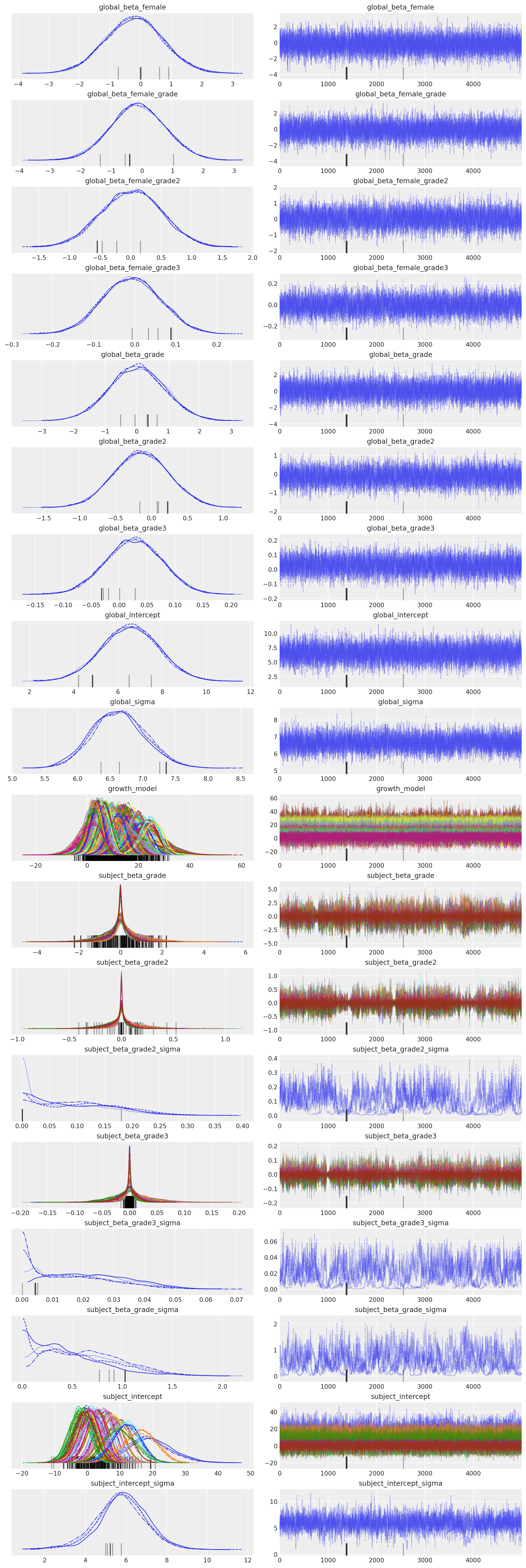
az.summary(
    idata_m7,
    var_names=[
        "global_intercept",
        "global_sigma",
        "global_beta_grade",
        "global_beta_grade2",
        "subject_intercept_sigma",
        "subject_beta_grade_sigma",
        "subject_beta_grade2_sigma",
        "subject_beta_grade3_sigma",
        "global_beta_female",
        "global_beta_female_grade",
        "global_beta_female_grade2",
        "global_beta_female_grade3",
    ],
)
| mean | sd | hdi_3% | hdi_97% | mcse_mean | mcse_sd | ess_bulk | ess_tail | r_hat | |
|---|---|---|---|---|---|---|---|---|---|
| global_intercept | 6.557 | 1.297 | 4.027 | 8.916 | 0.016 | 0.011 | 6847.0 | 10276.0 | 1.00 |
| global_sigma | 6.633 | 0.408 | 5.871 | 7.393 | 0.010 | 0.007 | 1777.0 | 8061.0 | 1.00 |
| global_beta_grade | 0.009 | 0.878 | -1.577 | 1.735 | 0.011 | 0.008 | 6155.0 | 9098.0 | 1.00 |
| global_beta_grade2 | -0.139 | 0.390 | -0.840 | 0.621 | 0.006 | 0.004 | 4503.0 | 7911.0 | 1.00 |
| subject_intercept_sigma | 5.786 | 1.239 | 3.392 | 8.144 | 0.054 | 0.038 | 573.0 | 550.0 | 1.01 |
| subject_beta_grade_sigma | 0.552 | 0.379 | 0.003 | 1.218 | 0.047 | 0.033 | 50.0 | 166.0 | 1.07 |
| subject_beta_grade2_sigma | 0.098 | 0.072 | 0.001 | 0.220 | 0.009 | 0.006 | 60.0 | 171.0 | 1.07 |
| subject_beta_grade3_sigma | 0.019 | 0.013 | 0.000 | 0.042 | 0.001 | 0.001 | 131.0 | 111.0 | 1.05 |
| global_beta_female | -0.212 | 0.940 | -1.968 | 1.573 | 0.009 | 0.007 | 9904.0 | 10717.0 | 1.00 |
| global_beta_female_grade | -0.132 | 0.898 | -1.804 | 1.565 | 0.010 | 0.007 | 7308.0 | 10362.0 | 1.00 |
| global_beta_female_grade2 | 0.020 | 0.495 | -0.903 | 0.958 | 0.007 | 0.005 | 4831.0 | 7979.0 | 1.00 |
| global_beta_female_grade3 | -0.008 | 0.071 | -0.141 | 0.124 | 0.001 | 0.001 | 4882.0 | 8440.0 | 1.00 |
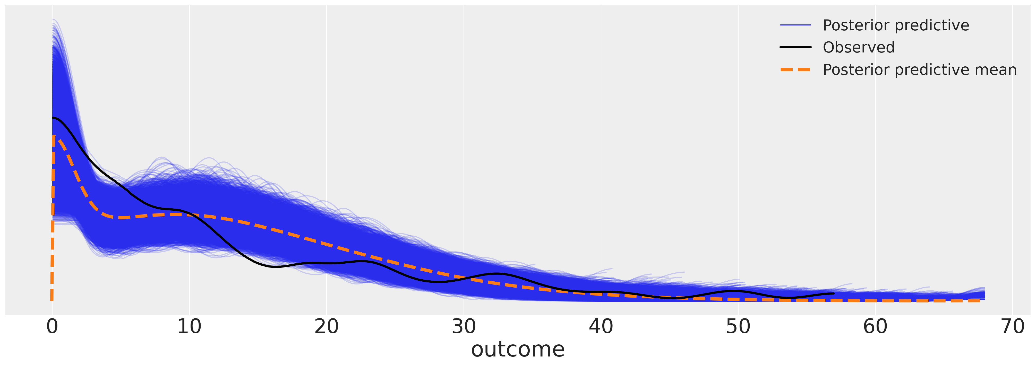
az.plot_ppc(idata_m7, figsize=(20, 7));
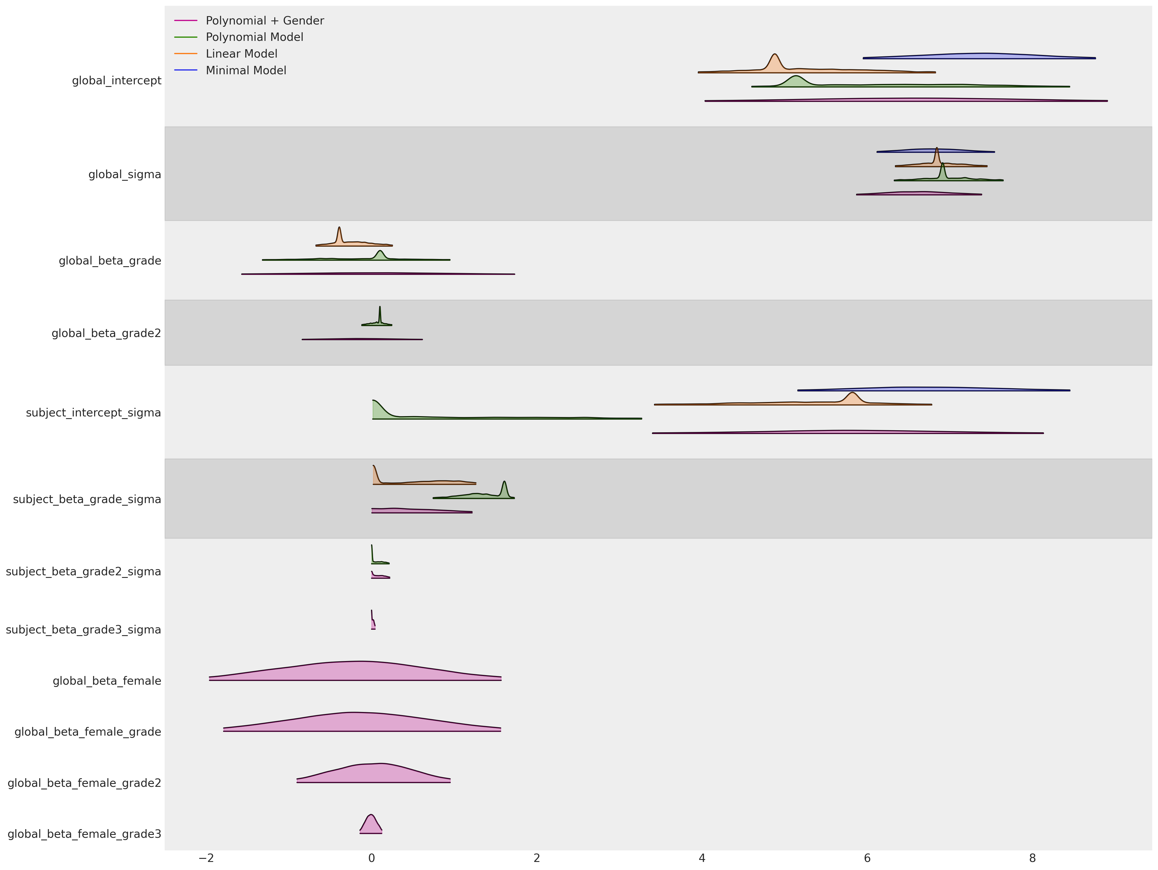
比较模型#
如上所述,我们将使用LOO比较各种模型的参数拟合和模型性能指标。
az.plot_forest(
    [idata_m4, idata_m5, idata_m6, idata_m7],
    model_names=["Minimal Model", "Linear Model", "Polynomial Model", "Polynomial + Gender"],
    var_names=[
        "global_intercept",
        "global_sigma",
        "global_beta_grade",
        "global_beta_grade2",
        "subject_intercept_sigma",
        "subject_beta_grade_sigma",
        "subject_beta_grade2_sigma",
        "subject_beta_grade3_sigma",
        "global_beta_female",
        "global_beta_female_grade",
        "global_beta_female_grade2",
        "global_beta_female_grade3",
    ],
    figsize=(20, 15),
    kind="ridgeplot",
    combined=True,
    coords={"ids": [1, 2, 30]},
    ridgeplot_alpha=0.3,
);
compare = az.compare(
    {
        "Minimal Model": idata_m4,
        "Linear Model": idata_m5,
        "Polynomial Model": idata_m6,
        "Polynomial + Gender": idata_m7,
    },
)
compare
/home/osvaldo/proyectos/00_BM/arviz-devs/arviz/arviz/stats/stats.py:795: UserWarning: Estimated shape parameter of Pareto distribution is greater than 0.70 for one or more samples. You should consider using a more robust model, this is because importance sampling is less likely to work well if the marginal posterior and LOO posterior are very different. This is more likely to happen with a non-robust model and highly influential observations.
  warnings.warn(
/home/osvaldo/proyectos/00_BM/arviz-devs/arviz/arviz/stats/stats.py:795: UserWarning: Estimated shape parameter of Pareto distribution is greater than 0.70 for one or more samples. You should consider using a more robust model, this is because importance sampling is less likely to work well if the marginal posterior and LOO posterior are very different. This is more likely to happen with a non-robust model and highly influential observations.
  warnings.warn(
/home/osvaldo/proyectos/00_BM/arviz-devs/arviz/arviz/stats/stats.py:795: UserWarning: Estimated shape parameter of Pareto distribution is greater than 0.70 for one or more samples. You should consider using a more robust model, this is because importance sampling is less likely to work well if the marginal posterior and LOO posterior are very different. This is more likely to happen with a non-robust model and highly influential observations.
  warnings.warn(
/home/osvaldo/proyectos/00_BM/arviz-devs/arviz/arviz/stats/stats.py:795: UserWarning: Estimated shape parameter of Pareto distribution is greater than 0.70 for one or more samples. You should consider using a more robust model, this is because importance sampling is less likely to work well if the marginal posterior and LOO posterior are very different. This is more likely to happen with a non-robust model and highly influential observations.
  warnings.warn(
| rank | elpd_loo | p_loo | elpd_diff | weight | se | dse | warning | scale | |
|---|---|---|---|---|---|---|---|---|---|
| Linear Model | 0 | -913.492285 | 32.270139 | 0.000000 | 8.146420e-01 | 13.556027 | 0.000000 | True | log |
| Polynomial + Gender | 1 | -915.895242 | 49.043791 | 2.402957 | 8.394507e-16 | 13.449388 | 2.597256 | True | log |
| Minimal Model | 2 | -917.384833 | 33.632784 | 3.892548 | 7.475052e-16 | 13.823280 | 2.375968 | True | log |
| Polynomial Model | 3 | -921.859743 | 27.035846 | 8.367458 | 1.853580e-01 | 14.762473 | 5.305436 | True | log |
az.plot_compare(compare, figsize=(10, 4));
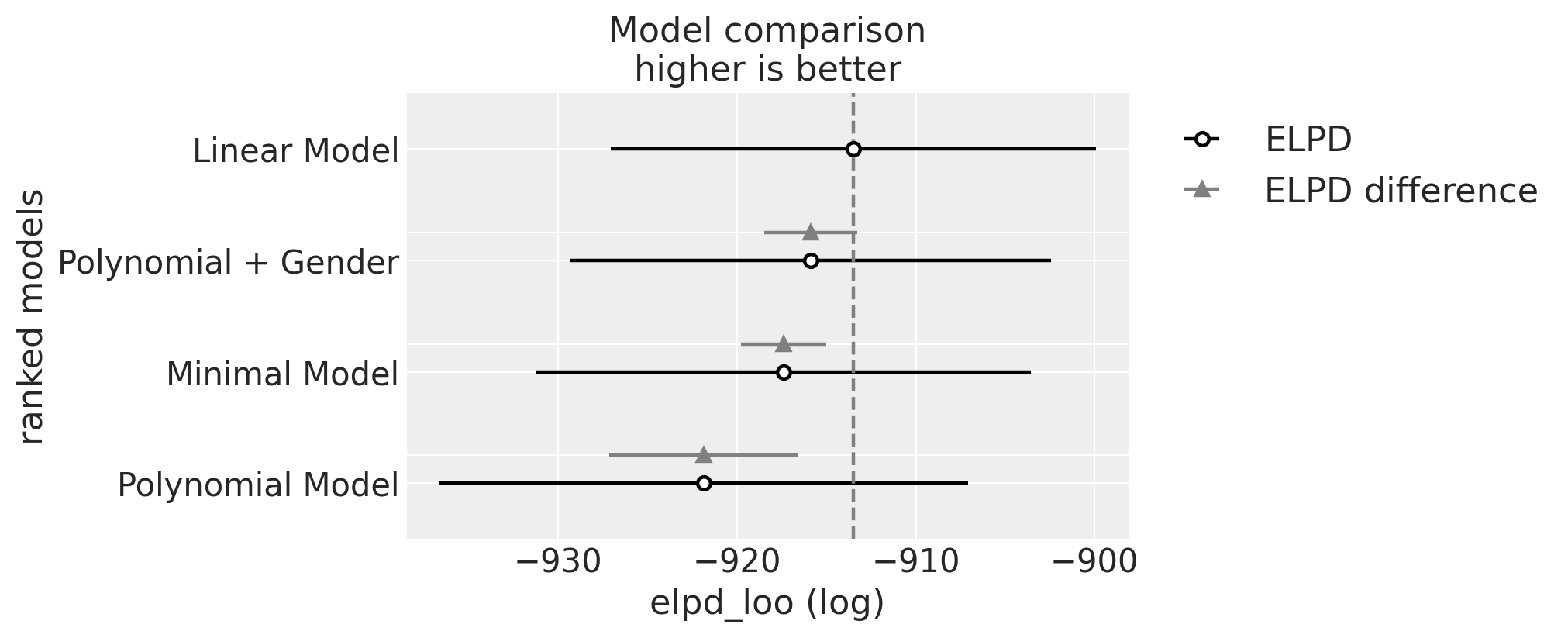
正如预期的那样,根据WAIC排名,我们最终的基于性别的模型被认为是最好的。但有点出人意料的是,具有固定轨迹的线性模型紧随其后。
绘制最终模型#
我们希望展示模型对多个个体的拟合情况以及在整个群体中隐含的总体趋势。
Show code cell source
def plot_individual(posterior, individual, female, ax):
    posterior = posterior.sel(ids=individual)
    time_xi = xr.DataArray(np.arange(7))
    i = posterior["global_intercept"].mean() + posterior["subject_intercept"]
    a = (posterior["global_beta_grade"].mean() + posterior["subject_beta_grade"]) * time_xi
    b = (posterior["global_beta_grade2"].mean() + posterior["subject_beta_grade2"]) * time_xi**2
    c = (posterior["global_beta_grade3"].mean() + posterior["subject_beta_grade3"]) * time_xi**3
    d = posterior["global_beta_female"].mean() * female + posterior["global_beta_female_grade"] * (
        time_xi * female
    )
    fit = i + a + b + c + d
    if female:
        color = "cyan"
    else:
        color = "slateblue"
    for i in range(len(fit)):
        ax.plot(time_xi, fit[i], color=color, alpha=0.1, linewidth=0.2)
    ax.plot(time_xi, fit.mean(axis=0), color="magenta")


mosaic = """BCDE
            AAAA
            FGHI"""
fig, axs = plt.subplot_mosaic(mosaic=mosaic, figsize=(20, 15))
axs = [axs[k] for k in axs.keys()]
posterior = az.extract(idata_m7.posterior, num_samples=4000)
intercept_group_specific = posterior["subject_intercept"].mean("ids")
slope_group_specific = posterior["subject_beta_grade"].mean("ids")
slope_group_specific_2 = posterior["subject_beta_grade2"].mean("ids")
slope_group_specific_3 = posterior["subject_beta_grade3"].mean("ids")
a = posterior["global_intercept"].mean() + intercept_group_specific
b = posterior["global_beta_grade"].mean() + slope_group_specific
c = posterior["global_beta_grade2"].mean() + slope_group_specific_2
d = posterior["global_beta_grade3"].mean() + slope_group_specific_3
e = posterior["global_beta_female"].mean()
f = posterior["global_beta_female_grade"].mean()

time_xi = xr.DataArray(np.arange(7))

axs[4].plot(
    time_xi,
    (a + b * time_xi + c * (time_xi**2) + d * (time_xi**3) + e * 1 + f * (1 * time_xi)).T,
    color="cyan",
    linewidth=2,
    alpha=0.1,
)
axs[4].plot(
    time_xi,
    (a + b * time_xi + c * (time_xi**2) + d * (time_xi**3) + e * 0 + f * (0 * time_xi)).T,
    color="slateblue",
    alpha=0.1,
    linewidth=2,
)
axs[4].plot(
    time_xi,
    (
        a.mean()
        + b.mean() * time_xi
        + c.mean() * (time_xi**2)
        + d.mean() * (time_xi**3)
        + e * 0
        + f * (0 * time_xi)
    ),
    color="red",
    lw=2,
    label="Expected Growth Trajectory - Male",
)

axs[4].plot(
    time_xi,
    (
        a.mean()
        + b.mean() * time_xi
        + c.mean() * (time_xi**2)
        + d.mean() * (time_xi**3)
        + e * 1
        + f * (1 * time_xi)
    ),
    color="darkblue",
    lw=2,
    label="Expected Growth Trajectory - Female",
)

for indx, id in zip([0, 1, 2, 3, 5, 6, 7, 8], [2, 8, 10, 30, 34, 40, 9, 11]):
    female = df_external[df_external["ID"] == id]["FEMALE"].unique()[0] == 1
    plot_individual(posterior, id, female, axs[indx])
    axs[indx].plot(
        df_external[df_external["ID"] == id]["GRADE"],
        df_external[df_external["ID"] == id]["EXTERNAL"],
        "o",
        color="black",
        label="Observed",
    )
    axs[indx].set_title(f"Within the Individual {id} Uncertainty")
    axs[indx].legend()


axs[4].set_ylabel("Externalising Score")
axs[4].set_xlabel("Time in Grade")
axs[4].legend()
axs[4].set_title("Between Individual Trajectories \n By Gender", fontsize=20);
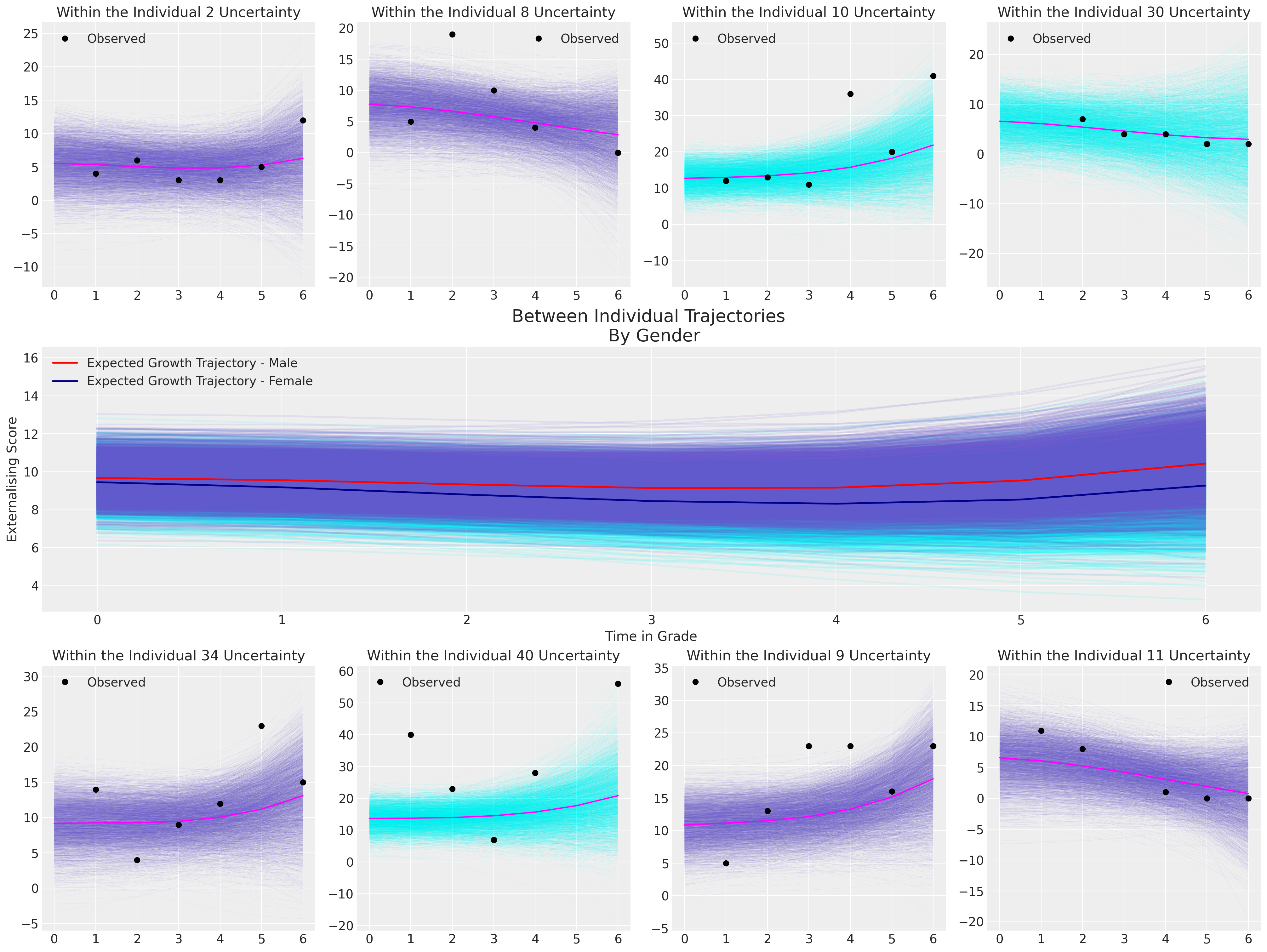
这个最终模型的含义表明,男性和女性在可能的成长轨迹上存在非常微小的差异,而且外化行为随时间变化的水平变化也非常小,但在6年级时趋于上升。请注意,对于个体40,模型拟合无法捕捉到观察数据中的剧烈波动。这是由于收缩效应,它将我们的截距项强烈地拉向全局平均值。这是一个很好的提醒,模型是为了泛化,而不是个体轨迹的完美表示。
结论#
我们现在已经了解了如何将贝叶斯分层模型应用于研究并探讨关于随时间变化的问题。我们看到了贝叶斯工作流的灵活性如何能够结合不同的先验和模型规范组合,以捕捉数据生成过程的细微差别。至关重要的是,我们看到了如何在个体内部视角和个体间模型的含义之间进行转换,同时评估模型对数据的忠实度。在面板数据背景下评估因果推断问题存在一些细微的问题,但也很明显,纵向建模使我们能够以系统化和有原则的方式梳理个体差异的复杂性。
这些是用于捕捉和评估变化模式以在队列内和队列间进行比较的强大模型。在没有随机对照试验或其他设计实验和准实验模式的情况下,这种类型的面板数据分析是你能从观察数据中得出因果结论(至少部分地考虑到个体治疗结果的异质性)的最接近的方法。
参考资料#
朱迪思·辛格 .D 和 约翰·威利特 .B. 应用纵向数据分析。牛津大学出版社,2003年。
A. 所罗门·库尔兹. 应用纵向数据分析在brms和tidyverse中. Bookdown, 2021. URL: https://bookdown.org/content/4253/.
水印#
%load_ext watermark
%watermark -n -u -v -iv -w -p pytensor
Last updated: Sat Aug 17 2024

Python implementation: CPython
Python version       : 3.11.5
IPython version      : 8.16.1

pytensor: 2.25.2

xarray     : 2023.10.1
matplotlib : 3.8.4
statsmodels: 0.14.2
arviz      : 0.19.0.dev0
pymc       : 5.16.2+20.g747fda319
numpy      : 1.24.4
bambi      : 0.14.0
pandas     : 2.1.2
preliz     : 0.9.0

Watermark: 2.4.3
许可证声明#
本示例库中的所有笔记本均在MIT许可证下提供,该许可证允许修改和重新分发,前提是保留版权和许可证声明。
引用 PyMC 示例#
要引用此笔记本,请使用Zenodo为pymc-examples仓库提供的DOI。
重要
许多笔记本是从其他来源改编的:博客、书籍……在这种情况下,您应该引用原始来源。
同时记得引用代码中使用的相关库。
这是一个BibTeX的引用模板:
@incollection{citekey,
  author    = "<notebook authors, see above>",
  title     = "<notebook title>",
  editor    = "PyMC Team",
  booktitle = "PyMC examples",
  doi       = "10.5281/zenodo.5654871"
}
渲染后可能看起来像: