


使用PyMC进行变分推断简介#
计算贝叶斯模型后验量的最常见策略是通过采样,特别是马尔可夫链蒙特卡洛(MCMC)算法。尽管采样算法及其相关计算在性能和效率方面不断改进,但MCMC方法在数据规模上仍然扩展性较差,对于超过几千个观测值的情况变得不可行。一种更具扩展性的替代方法是变分推断(VI),它将计算后验分布的问题重新表述为一个优化问题。
在 PyMC 中,变分推断 API 专注于通过一系列现代算法来近似后验分布。该模块可以应用的常见用例包括:
从模型后验中采样并计算任意表达式
进行期望、方差和其他统计量的蒙特卡罗近似
移除对PyMC随机节点的符号依赖并评估表达式(使用
eval)提供一个连接到任意 PyTensor 代码的桥梁
%matplotlib inline
import arviz as az
import matplotlib.pyplot as plt
import numpy as np
import pymc as pm
import pytensor
import seaborn as sns

np.random.seed(42)
分布近似#
统计学中有几种方法使用更简单的分布来近似更复杂的分布。也许最著名的例子是拉普拉斯(正态)近似。这涉及构建目标后验的泰勒级数,但仅保留二次项,并使用这些项来构建多元正态近似。
同样地,变分推断是另一种分布近似方法,其中,不是利用泰勒级数,而是选择某种近似分布类别,并优化其参数,使得生成的分布尽可能接近后验分布。本质上,变分推断是一种确定性近似方法,它对感兴趣的密度进行约束,然后使用优化方法从该约束集中进行选择。
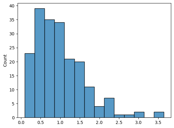
gamma_data = np.random.gamma(2, 0.5, size=200)
sns.histplot(gamma_data);
with pm.Model() as gamma_model:
    alpha = pm.Exponential("alpha", 0.1)
    beta = pm.Exponential("beta", 0.1)

    y = pm.Gamma("y", alpha, beta, observed=gamma_data)
with gamma_model:
    # mean_field = pm.fit()
    mean_field = pm.fit(obj_optimizer=pm.adagrad_window(learning_rate=1e-2))
Finished [100%]: Average Loss = 169.87
with gamma_model:
    trace = pm.sample()
Auto-assigning NUTS sampler...
Initializing NUTS using jitter+adapt_diag...
Multiprocess sampling (4 chains in 4 jobs)
NUTS: [alpha, beta]
Sampling 4 chains for 1_000 tune and 1_000 draw iterations (4_000 + 4_000 draws total) took 3 seconds.
mean_field
<pymc.variational.approximations.MeanField at 0x7fca20419e50>
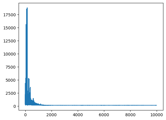
plt.plot(mean_field.hist);
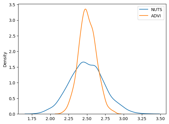
approx_sample = mean_field.sample(1000)
sns.kdeplot(trace.posterior["alpha"].values.flatten(), label="NUTS")
sns.kdeplot(approx_sample.posterior["alpha"].values.flatten(), label="ADVI")
plt.legend();
基本设置#
我们不需要复杂的模型来使用VI API;让我们从一个简单的混合模型开始:
w = np.array([0.2, 0.8])
mu = np.array([-0.3, 0.5])
sd = np.array([0.1, 0.1])

with pm.Model() as model:
    x = pm.NormalMixture("x", w=w, mu=mu, sigma=sd)
    x2 = x**2
    sin_x = pm.math.sin(x)
我们无法为此模型计算解析期望。然而,我们可以使用马尔可夫链蒙特卡罗方法获得一个近似值;让我们首先使用NUTS。
为了允许保存表达式的样本,我们需要将它们包装在 Deterministic 对象中:
with model:
    pm.Deterministic("x2", x2)
    pm.Deterministic("sin_x", sin_x)
with model:
    trace = pm.sample(5000)
Auto-assigning NUTS sampler...
Initializing NUTS using jitter+adapt_diag...
Multiprocess sampling (4 chains in 4 jobs)
NUTS: [x]
Sampling 4 chains for 1_000 tune and 5_000 draw iterations (4_000 + 20_000 draws total) took 5 seconds.
az.plot_trace(trace);
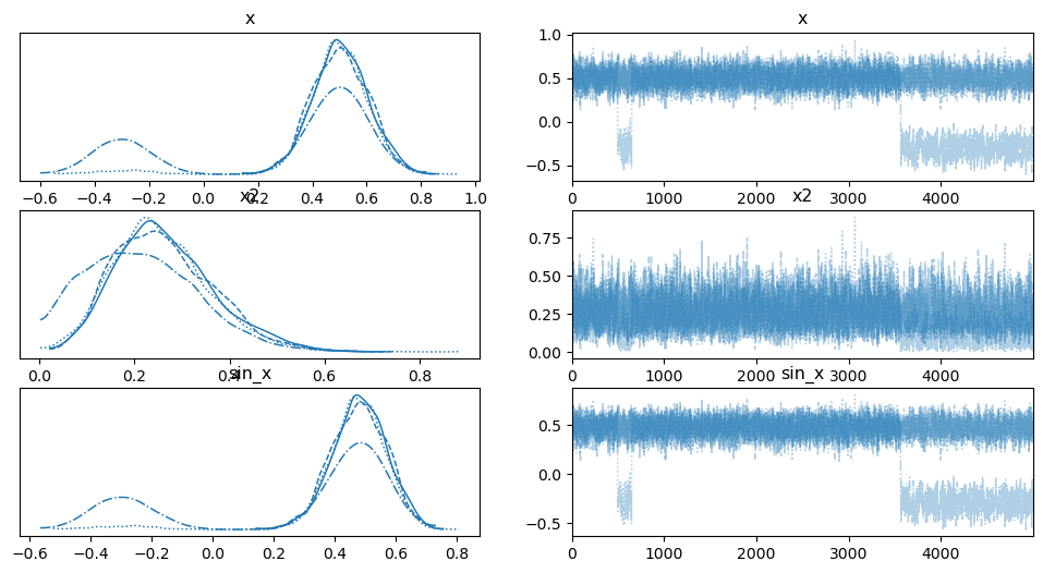
以上是 \(x^2\) 和 \(sin(x)\) 的轨迹。我们可以看到这个模型中存在明显的多模态性。一个缺点是,你需要提前知道你想要在轨迹中看到什么,并将其用 Deterministic 包裹起来。
VI API 采用了一种不同的方法:您从模型中获取推断,然后基于该模型计算表达式。
让我们使用相同的模型:
with pm.Model() as model:
    x = pm.NormalMixture("x", w=w, mu=mu, sigma=sd)
    x2 = x**2
    sin_x = pm.math.sin(x)
这里我们将使用自动微分变分推断(ADVI)。
with model:
    mean_field = pm.fit(method="advi")
Finished [100%]: Average Loss = 2.216
az.plot_posterior(mean_field.sample(1000), color="LightSeaGreen");
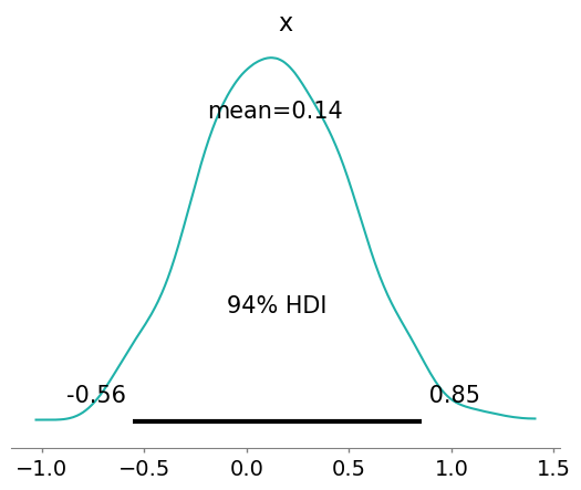
请注意,ADVI未能近似多模态分布,因为它使用的是具有单一模式的正态分布。
检查收敛性#
让我们使用 CheckParametersConvergence 的默认参数,因为它们看起来是合理的。
from pymc.variational.callbacks import CheckParametersConvergence

with model:
    mean_field = pm.fit(method="advi", callbacks=[CheckParametersConvergence()])
Finished [100%]: Average Loss = 2.239
我们可以通过.hist属性访问推理历史。
plt.plot(mean_field.hist);
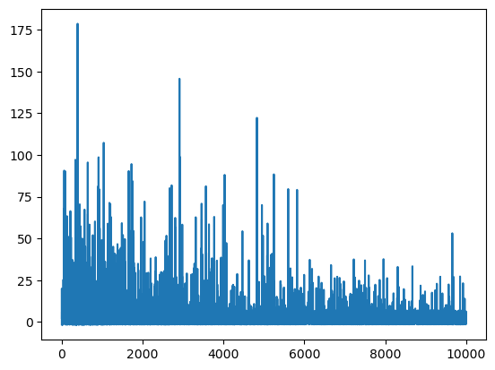
这不是一个好的收敛图,尽管我们运行了很多次迭代。原因是ADVI近似的均值接近于零,因此采用相对差异(默认方法)来检查收敛性是不稳定的。
with model:
    mean_field = pm.fit(
        method="advi", callbacks=[pm.callbacks.CheckParametersConvergence(diff="absolute")]
    )
Convergence achieved at 6200
Interrupted at 6,199 [61%]: Average Loss = 4.3808
plt.plot(mean_field.hist);
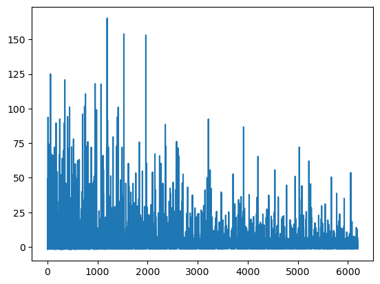
这样好多了!我们在不到5000次迭代后就达到了收敛。
跟踪参数#
另一个有用的回调允许用户跟踪参数。它允许在推理过程中跟踪任意统计数据,尽管它可能会占用大量内存。使用fit函数,我们在推理之前无法直接访问近似值。然而,跟踪参数需要访问近似值。我们可以通过使用面向对象(OO)API进行推理来绕过这一限制。
advi.approx
<pymc.variational.approximations.MeanField at 0x7fca1daee6a0>
不同的近似方法有不同的超参数。在均值场ADVI中,我们有\(\rho\)和\(\mu\)(灵感来自Bayes by BackProp)。
advi.approx.shared_params
{'mu': mu, 'rho': rho}
有一些方便的快捷方式可以访问与近似相关的统计数据。例如,这在为NUTS采样指定质量矩阵时非常有用:
advi.approx.mean.eval(), advi.approx.std.eval()
(array([0.34]), array([0.69314718]))
我们可以将这些统计数据整合到 Tracker 回调中。
tracker = pm.callbacks.Tracker(
    mean=advi.approx.mean.eval,  # callable that returns mean
    std=advi.approx.std.eval,  # callable that returns std
)
现在,调用 advi.fit 将会在运行过程中记录近似的均值和标准差。
approx = advi.fit(20000, callbacks=[tracker])
Finished [100%]: Average Loss = 2.2862
我们现在可以绘制证据下界和参数轨迹:
fig = plt.figure(figsize=(16, 9))
mu_ax = fig.add_subplot(221)
std_ax = fig.add_subplot(222)
hist_ax = fig.add_subplot(212)
mu_ax.plot(tracker["mean"])
mu_ax.set_title("Mean track")
std_ax.plot(tracker["std"])
std_ax.set_title("Std track")
hist_ax.plot(advi.hist)
hist_ax.set_title("Negative ELBO track");
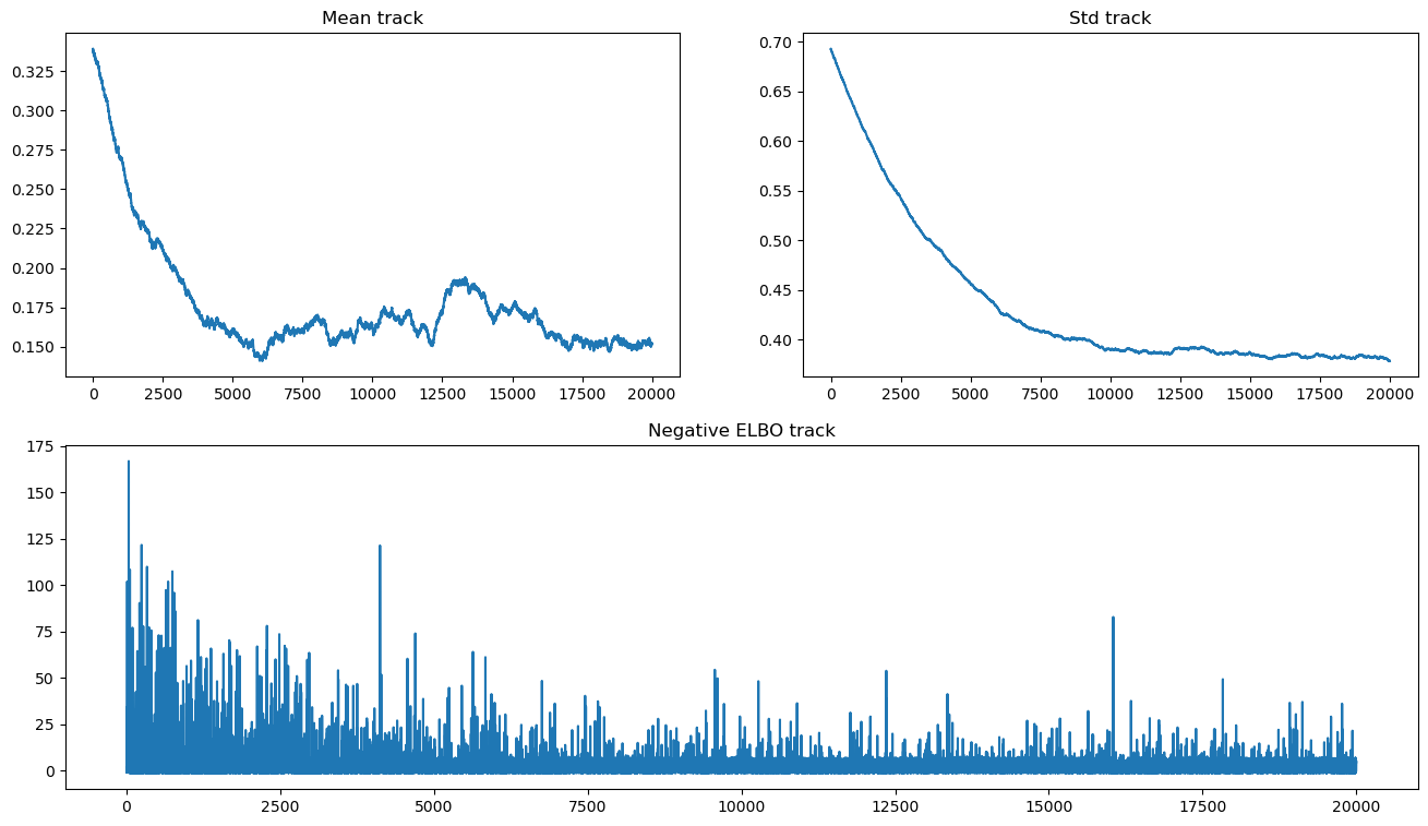
请注意,均值存在收敛问题,并且缺乏收敛似乎并不会显著改变ELBO轨迹。由于我们使用的是OO API,我们可以运行更长时间的近似计算,直到达到收敛。
advi.refine(100_000)
Finished [100%]: Average Loss = 2.1363
让我们来看一下:
fig = plt.figure(figsize=(16, 9))
mu_ax = fig.add_subplot(221)
std_ax = fig.add_subplot(222)
hist_ax = fig.add_subplot(212)
mu_ax.plot(tracker["mean"])
mu_ax.set_title("Mean track")
std_ax.plot(tracker["std"])
std_ax.set_title("Std track")
hist_ax.plot(advi.hist)
hist_ax.set_title("Negative ELBO track");
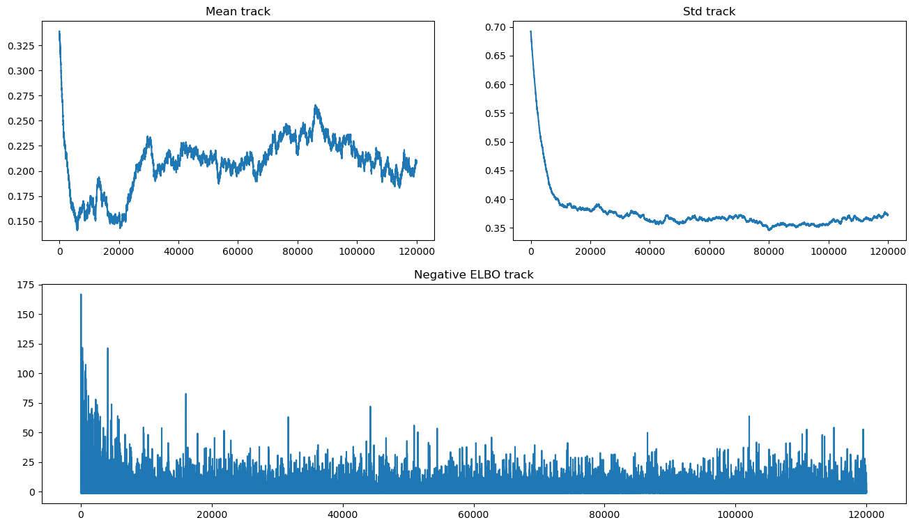
我们仍然看到缺乏收敛的证据,因为均值已经退化为随机游走。这可能是由于选择了不适合的推理算法所导致的。无论如何,它是不稳定的,即使使用不同的随机种子,也可能产生非常不同的结果。
让我们将结果与NUTS输出进行比较:
sns.kdeplot(trace.posterior["x"].values.flatten(), label="NUTS")
sns.kdeplot(approx.sample(20000).posterior["x"].values.flatten(), label="ADVI")
plt.legend();
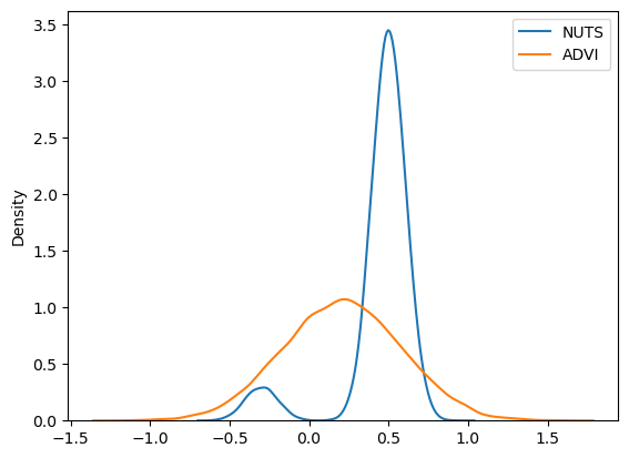
再次,我们看到ADVI无法处理多模态性;我们可以改用SVGD,它基于大量粒子生成一个近似值。
sns.kdeplot(trace.posterior["x"].values.flatten(), label="NUTS")
sns.kdeplot(approx.sample(10000).posterior["x"].values.flatten(), label="ADVI")
sns.kdeplot(svgd_approx.sample(2000).posterior["x"].values.flatten(), label="SVGD")
plt.legend();
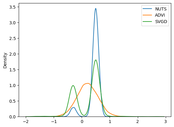
这解决了问题,因为我们现在使用SVGD得到了一个多模态近似。
通过这种方法,可以使用这种变分近似来计算参数的任意函数。例如,我们可以计算 \(x^2\) 和 \(sin(x)\),就像在NUTS模型中一样。
# recall x ~ NormalMixture
a = x**2
b = pm.math.sin(x)
要使用近似值评估这些表达式,我们需要 approx.sample_node。
a_sample = svgd_approx.sample_node(a)
a_sample.eval()
array(0.06251754)
a_sample.eval()
array(0.06251754)
a_sample.eval()
array(0.06251754)
每次调用都会从同一个节点得到不同的值。这是因为它是随机的。
通过应用替换,我们现在已经摆脱了对 PyMC 模型的依赖;相反,我们现在依赖于近似值。改变它将改变随机节点的分布:
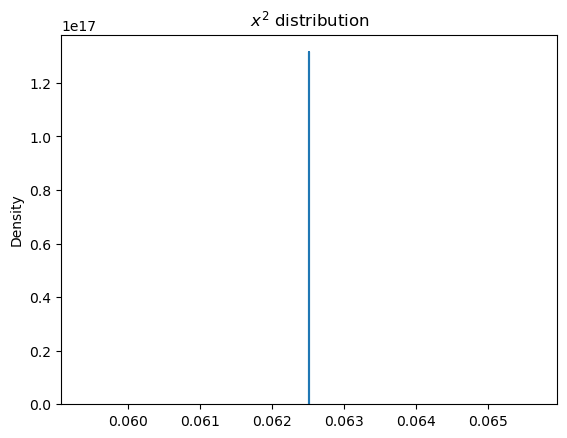
有一种更方便的方式可以一次性获取大量样本:sample_node
a_samples = svgd_approx.sample_node(a, size=1000)
sns.kdeplot(a_samples.eval())
plt.title("$x^2$ distribution");
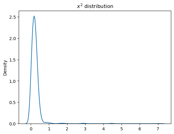
函数 sample_node 包含一个额外的维度,因此计算期望或方差时需要指定 axis=0。
a_samples.var(0).eval() # variance
array(0.13313996)
a_samples.mean(0).eval() # mean
array(0.24540344)
也可以指定一个符号样本大小:
a_samples_i.eval({i: 100}).shape
(100,)
a_samples_i.eval({i: 10000}).shape
(10000,)
不幸的是,大小必须是一个标量值。
多标签逻辑回归#
让我们以著名的鸢尾花数据集来说明Tracker的使用。我们将尝试多标签分类,并计算预期的准确率分数作为诊断。
import pandas as pd

from sklearn.datasets import load_iris
from sklearn.model_selection import train_test_split

X, y = load_iris(return_X_y=True)
X_train, X_test, y_train, y_test = train_test_split(X, y)

这里一个相对简单的模型就足够了,因为这些类别大致上是线性可分的;我们将拟合多项逻辑回归。
Xt = pytensor.shared(X_train)
yt = pytensor.shared(y_train)

with pm.Model() as iris_model:
    # Coefficients for features
    β = pm.Normal("β", 0, sigma=1e2, shape=(4, 3))
    # Transoform to unit interval
    a = pm.Normal("a", sigma=1e4, shape=(3,))
    p = pt.special.softmax(Xt.dot(β) + a, axis=-1)

    observed = pm.Categorical("obs", p=p, observed=yt)
在实践中应用替换#
PyMC 模型具有潜在变量的符号输入。要评估需要了解潜在变量的表达式,需要提供固定值。我们可以为此目的使用 VI 近似值。函数 sample_node 消除了符号依赖性。
sample_node 将在每一步使用整个分布,因此我们将在这里使用它。我们可以在单个函数调用中应用更多的替换,使用替换函数中的 more_replacements 关键字参数。
提示: 在调用
fit时,您也可以使用more_replacements参数:
pm.fit(more_replacements={full_data: minibatch_data})
inference.fit(more_replacements={full_data: minibatch_data})
with iris_model:
    # We'll use SVGD
    inference = pm.SVGD(n_particles=500, jitter=1)

    # Local reference to approximation
    approx = inference.approx

    # Here we need `more_replacements` to change train_set to test_set
    test_probs = approx.sample_node(p, more_replacements={Xt: X_test}, size=100)

    # For train set no more replacements needed
    train_probs = approx.sample_node(p)
通过应用上述代码,我们现在为每个观测值获得了100个采样概率(sample_node的默认数量为None)。
接下来我们为采样的准确率分数创建符号表达式:
Tracker 期望传入可调用对象,因此我们可以传递 PyTensor 节点的 .eval 方法,该方法本身就是一个函数。
对该函数的调用会被缓存,以便可以重复使用。
eval_tracker = pm.callbacks.Tracker(
    test_accuracy=test_accuracy.eval, train_accuracy=train_accuracy.eval
)
inference.fit(100, callbacks=[eval_tracker]);
_, ax = plt.subplots(1, 1)
df = pd.DataFrame(eval_tracker["test_accuracy"]).T.melt()
sns.lineplot(x="variable", y="value", data=df, color="red", ax=ax)
ax.plot(eval_tracker["train_accuracy"], color="blue")
ax.set_xlabel("epoch")
plt.legend(["test_accuracy", "train_accuracy"])
plt.title("Training Progress");
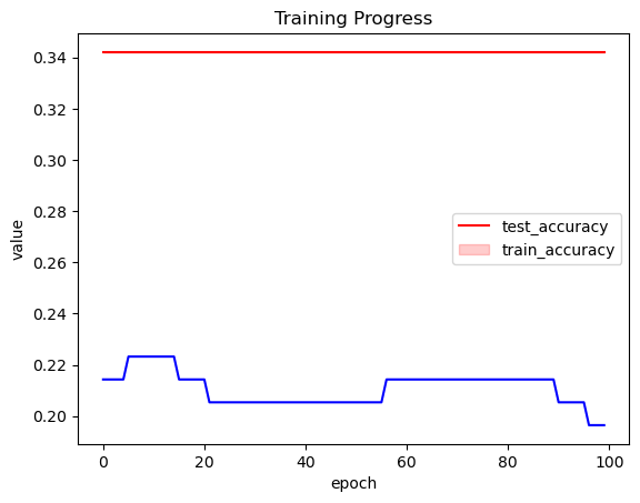
训练在这里似乎不起作用。让我们使用不同的优化器并提高学习率。
inference.fit(400, obj_optimizer=pm.adamax(learning_rate=0.1), callbacks=[eval_tracker]);
_, ax = plt.subplots(1, 1)
df = pd.DataFrame(np.asarray(eval_tracker["test_accuracy"])).T.melt()
sns.lineplot(x="variable", y="value", data=df, color="red", ax=ax)
ax.plot(eval_tracker["train_accuracy"], color="blue")
ax.set_xlabel("epoch")
plt.legend(["test_accuracy", "train_accuracy"])
plt.title("Training Progress");
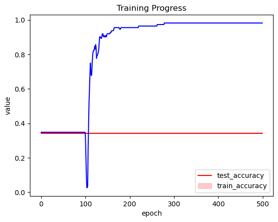
这好多了!
因此,Tracker 允许我们监控我们的近似值并选择良好的训练计划。
小批量#
在处理大型数据集时,使用小批量训练可以显著加快并提高近似性能。大型数据集对梯度计算的成本很高。
在PyMC中有一个很好的API来处理这些情况,它可以通过pm.Minibatch类来使用。minibatch只是一个高度专业化的PyTensor张量。
为了演示,让我们模拟大量数据:
# Raw values
data = np.random.rand(40000, 100)
# Scaled values
data *= np.random.randint(1, 10, size=(100,))
# Shifted values
data += np.random.rand(100) * 10
作为对比,让我们拟合一个不使用小批量处理的模型:
只是为了好玩,让我们创建一个自定义的特殊用途回调函数来停止缓慢的优化。这里我们定义了一个回调函数,当近似计算运行得太慢时会导致硬停止:
def stop_after_10(approx, loss_history, i):
    if (i > 0) and (i % 10) == 0:
        raise StopIteration("I was slow, sorry")
with model:
    advifit = pm.fit(callbacks=[stop_after_10])
---------------------------------------------------------------------------
KeyboardInterrupt                         Traceback (most recent call last)
Cell In[66], line 2
      1 with model:
----> 2     advifit = pm.fit(callbacks=[stop_after_10])

File ~/mambaforge/envs/pie/lib/python3.9/site-packages/pymc/variational/inference.py:747, in fit(n, method, model, random_seed, start, start_sigma, inf_kwargs, **kwargs)
    745 else:
    746     raise TypeError(f"method should be one of {set(_select.keys())} or Inference instance")
--> 747 return inference.fit(n, **kwargs)

File ~/mambaforge/envs/pie/lib/python3.9/site-packages/pymc/variational/inference.py:138, in Inference.fit(self, n, score, callbacks, progressbar, **kwargs)
    136     callbacks = []
    137 score = self._maybe_score(score)
--> 138 step_func = self.objective.step_function(score=score, **kwargs)
    139 if progressbar:
    140     progress = progress_bar(range(n), display=progressbar)

File ~/mambaforge/envs/pie/lib/python3.9/site-packages/pytensor/configparser.py:47, in _ChangeFlagsDecorator.__call__.<locals>.res(*args, **kwargs)
     44 @wraps(f)
     45 def res(*args, **kwargs):
     46     with self:
---> 47         return f(*args, **kwargs)

File ~/mambaforge/envs/pie/lib/python3.9/site-packages/pymc/variational/opvi.py:387, in ObjectiveFunction.step_function(self, obj_n_mc, tf_n_mc, obj_optimizer, test_optimizer, more_obj_params, more_tf_params, more_updates, more_replacements, total_grad_norm_constraint, score, fn_kwargs)
    385 seed = self.approx.rng.randint(2**30, dtype=np.int64)
    386 if score:
--> 387     step_fn = compile_pymc([], updates.loss, updates=updates, random_seed=seed, **fn_kwargs)
    388 else:
    389     step_fn = compile_pymc([], [], updates=updates, random_seed=seed, **fn_kwargs)

File ~/mambaforge/envs/pie/lib/python3.9/site-packages/pymc/pytensorf.py:1121, in compile_pymc(inputs, outputs, random_seed, mode, **kwargs)
   1119 opt_qry = mode.provided_optimizer.including("random_make_inplace", check_parameter_opt)
   1120 mode = Mode(linker=mode.linker, optimizer=opt_qry)
-> 1121 pytensor_function = pytensor.function(
   1122     inputs,
   1123     outputs,
   1124     updates={**rng_updates, **kwargs.pop("updates", {})},
   1125     mode=mode,
   1126     **kwargs,
   1127 )
   1128 return pytensor_function

File ~/mambaforge/envs/pie/lib/python3.9/site-packages/pytensor/compile/function/__init__.py:315, in function(inputs, outputs, mode, updates, givens, no_default_updates, accept_inplace, name, rebuild_strict, allow_input_downcast, profile, on_unused_input)
    309     fn = orig_function(
    310         inputs, outputs, mode=mode, accept_inplace=accept_inplace, name=name
    311     )
    312 else:
    313     # note: pfunc will also call orig_function -- orig_function is
    314     #      a choke point that all compilation must pass through
--> 315     fn = pfunc(
    316         params=inputs,
    317         outputs=outputs,
    318         mode=mode,
    319         updates=updates,
    320         givens=givens,
    321         no_default_updates=no_default_updates,
    322         accept_inplace=accept_inplace,
    323         name=name,
    324         rebuild_strict=rebuild_strict,
    325         allow_input_downcast=allow_input_downcast,
    326         on_unused_input=on_unused_input,
    327         profile=profile,
    328         output_keys=output_keys,
    329     )
    330 return fn

File ~/mambaforge/envs/pie/lib/python3.9/site-packages/pytensor/compile/function/pfunc.py:367, in pfunc(params, outputs, mode, updates, givens, no_default_updates, accept_inplace, name, rebuild_strict, allow_input_downcast, profile, on_unused_input, output_keys, fgraph)
    353     profile = ProfileStats(message=profile)
    355 inputs, cloned_outputs = construct_pfunc_ins_and_outs(
    356     params,
    357     outputs,
   (...)
    364     fgraph=fgraph,
    365 )
--> 367 return orig_function(
    368     inputs,
    369     cloned_outputs,
    370     mode,
    371     accept_inplace=accept_inplace,
    372     name=name,
    373     profile=profile,
    374     on_unused_input=on_unused_input,
    375     output_keys=output_keys,
    376     fgraph=fgraph,
    377 )

File ~/mambaforge/envs/pie/lib/python3.9/site-packages/pytensor/compile/function/types.py:1766, in orig_function(inputs, outputs, mode, accept_inplace, name, profile, on_unused_input, output_keys, fgraph)
   1754     m = Maker(
   1755         inputs,
   1756         outputs,
   (...)
   1763         fgraph=fgraph,
   1764     )
   1765     with config.change_flags(compute_test_value="off"):
-> 1766         fn = m.create(defaults)
   1767 finally:
   1768     t2 = time.perf_counter()

File ~/mambaforge/envs/pie/lib/python3.9/site-packages/pytensor/compile/function/types.py:1659, in FunctionMaker.create(self, input_storage, trustme, storage_map)
   1656 start_import_time = pytensor.link.c.cmodule.import_time
   1658 with config.change_flags(traceback__limit=config.traceback__compile_limit):
-> 1659     _fn, _i, _o = self.linker.make_thunk(
   1660         input_storage=input_storage_lists, storage_map=storage_map
   1661     )
   1663 end_linker = time.perf_counter()
   1665 linker_time = end_linker - start_linker

File ~/mambaforge/envs/pie/lib/python3.9/site-packages/pytensor/link/basic.py:254, in LocalLinker.make_thunk(self, input_storage, output_storage, storage_map, **kwargs)
    247 def make_thunk(
    248     self,
    249     input_storage: Optional["InputStorageType"] = None,
   (...)
    252     **kwargs,
    253 ) -> Tuple["BasicThunkType", "InputStorageType", "OutputStorageType"]:
--> 254     return self.make_all(
    255         input_storage=input_storage,
    256         output_storage=output_storage,
    257         storage_map=storage_map,
    258     )[:3]

File ~/mambaforge/envs/pie/lib/python3.9/site-packages/pytensor/link/vm.py:1246, in VMLinker.make_all(self, profiler, input_storage, output_storage, storage_map)
   1241 thunk_start = time.perf_counter()
   1242 # no-recycling is done at each VM.__call__ So there is
   1243 # no need to cause duplicate c code by passing
   1244 # no_recycling here.
   1245 thunks.append(
-> 1246     node.op.make_thunk(node, storage_map, compute_map, [], impl=impl)
   1247 )
   1248 linker_make_thunk_time[node] = time.perf_counter() - thunk_start
   1249 if not hasattr(thunks[-1], "lazy"):
   1250     # We don't want all ops maker to think about lazy Ops.
   1251     # So if they didn't specify that its lazy or not, it isn't.
   1252     # If this member isn't present, it will crash later.

File ~/mambaforge/envs/pie/lib/python3.9/site-packages/pytensor/link/c/op.py:131, in COp.make_thunk(self, node, storage_map, compute_map, no_recycling, impl)
    127 self.prepare_node(
    128     node, storage_map=storage_map, compute_map=compute_map, impl="c"
    129 )
    130 try:
--> 131     return self.make_c_thunk(node, storage_map, compute_map, no_recycling)
    132 except (NotImplementedError, MethodNotDefined):
    133     # We requested the c code, so don't catch the error.
    134     if impl == "c":

File ~/mambaforge/envs/pie/lib/python3.9/site-packages/pytensor/link/c/op.py:96, in COp.make_c_thunk(self, node, storage_map, compute_map, no_recycling)
     94         print(f"Disabling C code for {self} due to unsupported float16")
     95         raise NotImplementedError("float16")
---> 96 outputs = cl.make_thunk(
     97     input_storage=node_input_storage, output_storage=node_output_storage
     98 )
     99 thunk, node_input_filters, node_output_filters = outputs
    101 @is_cthunk_wrapper_type
    102 def rval():

File ~/mambaforge/envs/pie/lib/python3.9/site-packages/pytensor/link/c/basic.py:1202, in CLinker.make_thunk(self, input_storage, output_storage, storage_map, cache, **kwargs)
   1167 """Compile this linker's `self.fgraph` and return a function that performs the computations.
   1168
   1169 The return values can be used as follows:
   (...)
   1199
   1200 """
   1201 init_tasks, tasks = self.get_init_tasks()
-> 1202 cthunk, module, in_storage, out_storage, error_storage = self.__compile__(
   1203     input_storage, output_storage, storage_map, cache
   1204 )
   1206 res = _CThunk(cthunk, init_tasks, tasks, error_storage, module)
   1207 res.nodes = self.node_order

File ~/mambaforge/envs/pie/lib/python3.9/site-packages/pytensor/link/c/basic.py:1122, in CLinker.__compile__(self, input_storage, output_storage, storage_map, cache)
   1120 input_storage = tuple(input_storage)
   1121 output_storage = tuple(output_storage)
-> 1122 thunk, module = self.cthunk_factory(
   1123     error_storage,
   1124     input_storage,
   1125     output_storage,
   1126     storage_map,
   1127     cache,
   1128 )
   1129 return (
   1130     thunk,
   1131     module,
   (...)
   1140     error_storage,
   1141 )

File ~/mambaforge/envs/pie/lib/python3.9/site-packages/pytensor/link/c/basic.py:1647, in CLinker.cthunk_factory(self, error_storage, in_storage, out_storage, storage_map, cache)
   1645     if cache is None:
   1646         cache = get_module_cache()
-> 1647     module = cache.module_from_key(key=key, lnk=self)
   1649 vars = self.inputs + self.outputs + self.orphans
   1650 # List of indices that should be ignored when passing the arguments
   1651 # (basically, everything that the previous call to uniq eliminated)

File ~/mambaforge/envs/pie/lib/python3.9/site-packages/pytensor/link/c/cmodule.py:1231, in ModuleCache.module_from_key(self, key, lnk)
   1229 try:
   1230     location = dlimport_workdir(self.dirname)
-> 1231     module = lnk.compile_cmodule(location)
   1232     name = module.__file__
   1233     assert name.startswith(location)

File ~/mambaforge/envs/pie/lib/python3.9/site-packages/pytensor/link/c/basic.py:1546, in CLinker.compile_cmodule(self, location)
   1544 try:
   1545     _logger.debug(f"LOCATION {location}")
-> 1546     module = c_compiler.compile_str(
   1547         module_name=mod.code_hash,
   1548         src_code=src_code,
   1549         location=location,
   1550         include_dirs=self.header_dirs(),
   1551         lib_dirs=self.lib_dirs(),
   1552         libs=libs,
   1553         preargs=preargs,
   1554     )
   1555 except Exception as e:
   1556     e.args += (str(self.fgraph),)

File ~/mambaforge/envs/pie/lib/python3.9/site-packages/pytensor/link/c/cmodule.py:2591, in GCC_compiler.compile_str(module_name, src_code, location, include_dirs, lib_dirs, libs, preargs, py_module, hide_symbols)
   2588     print(" ".join(cmd), file=sys.stderr)
   2590 try:
-> 2591     p_out = output_subprocess_Popen(cmd)
   2592     compile_stderr = p_out[1].decode()
   2593 except Exception:
   2594     # An exception can occur e.g. if `g++` is not found.

File ~/mambaforge/envs/pie/lib/python3.9/site-packages/pytensor/utils.py:261, in output_subprocess_Popen(command, **params)
    258 p = subprocess_Popen(command, **params)
    259 # we need to use communicate to make sure we don't deadlock around
    260 # the stdout/stderr pipe.
--> 261 out = p.communicate()
    262 return out + (p.returncode,)

File ~/mambaforge/envs/pie/lib/python3.9/subprocess.py:1130, in Popen.communicate(self, input, timeout)
   1127     endtime = None
   1129 try:
-> 1130     stdout, stderr = self._communicate(input, endtime, timeout)
   1131 except KeyboardInterrupt:
   1132     # https://bugs.python.org/issue25942
   1133     # See the detailed comment in .wait().
   1134     if timeout is not None:

File ~/mambaforge/envs/pie/lib/python3.9/subprocess.py:1977, in Popen._communicate(self, input, endtime, orig_timeout)
   1970     self._check_timeout(endtime, orig_timeout,
   1971                         stdout, stderr,
   1972                         skip_check_and_raise=True)
   1973     raise RuntimeError(  # Impossible :)
   1974         '_check_timeout(..., skip_check_and_raise=True) '
   1975         'failed to raise TimeoutExpired.')
-> 1977 ready = selector.select(timeout)
   1978 self._check_timeout(endtime, orig_timeout, stdout, stderr)
   1980 # XXX Rewrite these to use non-blocking I/O on the file
   1981 # objects; they are no longer using C stdio!

File ~/mambaforge/envs/pie/lib/python3.9/selectors.py:416, in _PollLikeSelector.select(self, timeout)
    414 ready = []
    415 try:
--> 416     fd_event_list = self._selector.poll(timeout)
    417 except InterruptedError:
    418     return ready

KeyboardInterrupt:
推理速度太慢,每次迭代需要几秒钟;拟合近似值将需要数小时!
现在让我们使用小批量数据。在每次迭代中,我们将抽取500个随机值:
记得在observed中设置
total_size
total_size 是一个重要的参数,它允许 PyMC 推断正确的密度重缩放方式。如果未设置此参数,您可能会得到完全错误的结果。更多信息请参阅 pm.Minibatch 的综合文档。
X = pm.Minibatch(data, batch_size=500)

with pm.Model() as model:
    mu = pm.Normal("mu", 0, sigma=1e5, shape=(100,))
    sd = pm.HalfNormal("sd", shape=(100,))
    likelihood = pm.Normal("likelihood", mu, sigma=sd, observed=X, total_size=data.shape)
with model:
    advifit = pm.fit()
Finished [100%]: Average Loss = 1.5101e+05
plt.plot(advifit.hist);
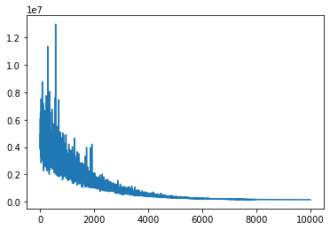
小批量推理的速度显著更快。在某些需要矩阵分解或模型非常宽的极端情况下,可能需要多维小批量。
这里是Minibatch的文档字符串,以说明如何对其进行自定义。
print(pm.Minibatch.__doc__)
Multidimensional minibatch that is pure TensorVariable

    Parameters
    ----------
    data: np.ndarray
        initial data
    batch_size: ``int`` or ``List[int|tuple(size, random_seed)]``
        batch size for inference, random seed is needed
        for child random generators
    dtype: ``str``
        cast data to specific type
    broadcastable: tuple[bool]
        change broadcastable pattern that defaults to ``(False, ) * ndim``
    name: ``str``
        name for tensor, defaults to "Minibatch"
    random_seed: ``int``
        random seed that is used by default
    update_shared_f: ``callable``
        returns :class:`ndarray` that will be carefully
        stored to underlying shared variable
        you can use it to change source of
        minibatches programmatically
    in_memory_size: ``int`` or ``List[int|slice|Ellipsis]``
        data size for storing in ``aesara.shared``

    Attributes
    ----------
    shared: shared tensor
        Used for storing data
    minibatch: minibatch tensor
        Used for training

    Notes
    -----
    Below is a common use case of Minibatch with variational inference.
    Importantly, we need to make PyMC "aware" that a minibatch is being used in inference.
    Otherwise, we will get the wrong :math:`logp` for the model.
    the density of the model ``logp`` that is affected by Minibatch. See more in the examples below.
    To do so, we need to pass the ``total_size`` parameter to the observed node, which correctly scales
    the density of the model ``logp`` that is affected by Minibatch. See more in the examples below.

    Examples
    --------
    Consider we have `data` as follows:

    >>> data = np.random.rand(100, 100)

    if we want a 1d slice of size 10 we do

    >>> x = Minibatch(data, batch_size=10)

    Note that your data is cast to ``floatX`` if it is not integer type
    But you still can add the ``dtype`` kwarg for :class:`Minibatch`
    if you need more control.

    If we want 10 sampled rows and columns
    ``[(size, seed), (size, seed)]`` we can use

    >>> x = Minibatch(data, batch_size=[(10, 42), (10, 42)], dtype='int32')
    >>> assert str(x.dtype) == 'int32'


    Or, more simply, we can use the default random seed = 42
    ``[size, size]``

    >>> x = Minibatch(data, batch_size=[10, 10])


    In the above, `x` is a regular :class:`TensorVariable` that supports any math operations:


    >>> assert x.eval().shape == (10, 10)


    You can pass the Minibatch `x` to your desired model:

    >>> with pm.Model() as model:
    ...     mu = pm.Flat('mu')
    ...     sigma = pm.HalfNormal('sigma')
    ...     lik = pm.Normal('lik', mu, sigma, observed=x, total_size=(100, 100))


    Then you can perform regular Variational Inference out of the box


    >>> with model:
    ...     approx = pm.fit()


    Important note: :class:``Minibatch`` has ``shared``, and ``minibatch`` attributes
    you can call later:

    >>> x.set_value(np.random.laplace(size=(100, 100)))

    and minibatches will be then from new storage
    it directly affects ``x.shared``.
    A less convenient convenient, but more explicit, way to achieve the same
    thing:

    >>> x.shared.set_value(pm.floatX(np.random.laplace(size=(100, 100))))

    The programmatic way to change storage is as follows
    I import ``partial`` for simplicity
    >>> from functools import partial
    >>> datagen = partial(np.random.laplace, size=(100, 100))
    >>> x = Minibatch(datagen(), batch_size=10, update_shared_f=datagen)
    >>> x.update_shared()

    To be more concrete about how we create a minibatch, here is a demo:
    1. create a shared variable

        >>> shared = aesara.shared(data)

    2. take a random slice of size 10:

        >>> ridx = pm.at_rng().uniform(size=(10,), low=0, high=data.shape[0]-1e-10).astype('int64')

    3) take the resulting slice:

        >>> minibatch = shared[ridx]

    That's done. Now you can use this minibatch somewhere else.
    You can see that the implementation does not require a fixed shape
    for the shared variable. Feel free to use that if needed.
    *FIXME: What is "that" which we can use here?  A fixed shape?  Should this say
    "but feel free to put a fixed shape on the shared variable, if appropriate?"*

    Suppose you need to make some replacements in the graph, e.g. change the minibatch to testdata

    >>> node = x ** 2  # arbitrary expressions on minibatch `x`
    >>> testdata = pm.floatX(np.random.laplace(size=(1000, 10)))

    Then you should create a `dict` with replacements:

    >>> replacements = {x: testdata}
    >>> rnode = aesara.clone_replace(node, replacements)
    >>> assert (testdata ** 2 == rnode.eval()).all()

    *FIXME: In the following, what is the **reason** to replace the Minibatch variable with
    its shared variable?  And in the following, the `rnode` is a **new** node, not a modification
    of a previously existing node, correct?*
    To replace a minibatch with its shared variable you should do
    the same things. The Minibatch variable is accessible through the `minibatch` attribute.
    For example

    >>> replacements = {x.minibatch: x.shared}
    >>> rnode = aesara.clone_replace(node, replacements)

    For more complex slices some more code is needed that can seem not so clear

    >>> moredata = np.random.rand(10, 20, 30, 40, 50)

    The default ``total_size`` that can be passed to PyMC random node
    is then ``(10, 20, 30, 40, 50)`` but can be less verbose in some cases

    1. Advanced indexing, ``total_size = (10, Ellipsis, 50)``

        >>> x = Minibatch(moredata, [2, Ellipsis, 10])

        We take the slice only for the first and last dimension

        >>> assert x.eval().shape == (2, 20, 30, 40, 10)

    2. Skipping a particular dimension, ``total_size = (10, None, 30)``:

        >>> x = Minibatch(moredata, [2, None, 20])
        >>> assert x.eval().shape == (2, 20, 20, 40, 50)

    3. Mixing both of these together, ``total_size = (10, None, 30, Ellipsis, 50)``:

        >>> x = Minibatch(moredata, [2, None, 20, Ellipsis, 10])
        >>> assert x.eval().shape == (2, 20, 20, 40, 10)
水印#
%load_ext watermark
%watermark -n -u -v -iv -w
Last updated: Sun Nov 20 2022

Python implementation: CPython
Python version       : 3.10.4
IPython version      : 8.4.0

sys       : 3.10.4 | packaged by conda-forge | (main, Mar 24 2022, 17:39:37) [Clang 12.0.1 ]
pymc      : 4.3.0
seaborn   : 0.11.2
arviz     : 0.13.0
numpy     : 1.22.4
matplotlib: 3.5.2
aesara    : 2.8.9+11.ge8eed6c18
pandas    : 1.4.2

Watermark: 2.3.1
许可证声明#
本示例库中的所有笔记本均在MIT许可证下提供,该许可证允许修改和重新分发,前提是保留版权和许可证声明。
引用 PyMC 示例#
要引用此笔记本,请使用Zenodo为pymc-examples仓库提供的DOI。
重要
许多笔记本是从其他来源改编的:博客、书籍……在这种情况下,您应该引用原始来源。
同时记得引用代码中使用的相关库。
这是一个BibTeX的引用模板:
@incollection{citekey,
  author    = "<notebook authors, see above>",
  title     = "<notebook title>",
  editor    = "PyMC Team",
  booktitle = "PyMC examples",
  doi       = "10.5281/zenodo.5654871"
}
渲染后可能看起来像: