比较算法：xNES与CMA-ES的案例#

在本教程中，我们将展示如何使用pygmo来比较两个UDAs的性能。我们制定了一个标准程序，这被认为是进行比较的最佳实践，并应在可能的情况下使用，即当算法具有明确定义的退出条件时。

我们以两个UDAs cmaes 和 xnes 为例。

两种算法都基于更新高斯分布的思想，该分布调节新样本的生成，但它们在更新规则上有所不同，xNES的更新规则可以说更优雅且更简洁。

为了比较算法，我们使用实验累积分布函数（ECDF）来描述在一定预算的函数评估内找到目标函数小于某个target的解的概率。估计这样的ECDF可以通过多次调用算法的evolve()方法（trials）并将结果组合成包含多次重启的单个运行来完成。

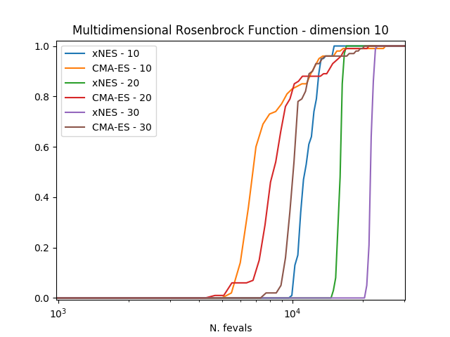
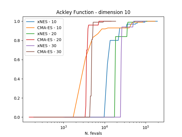
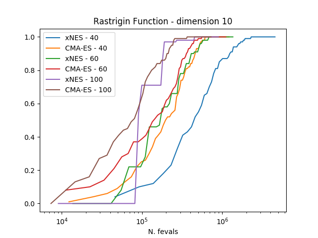
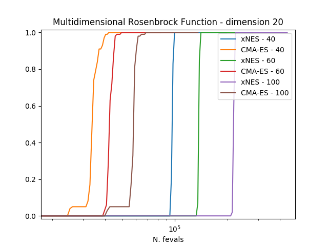
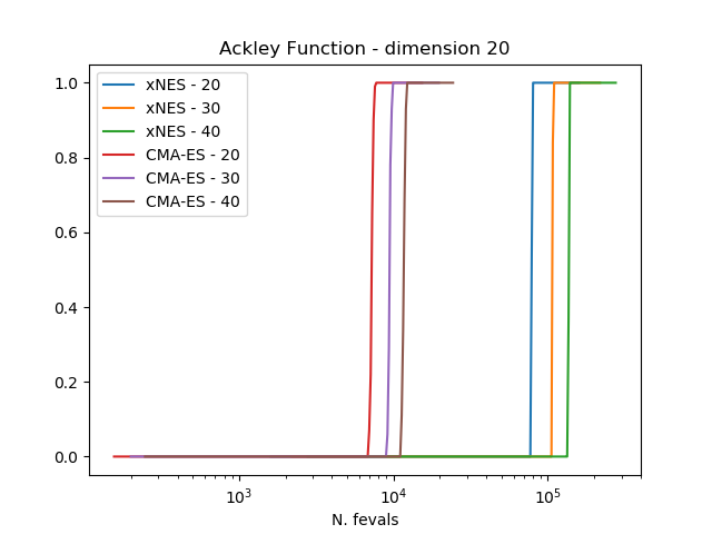
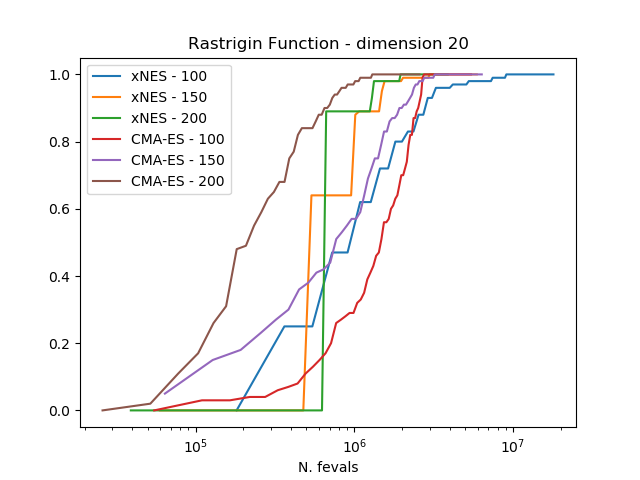
结果清楚地表明，在这三个考虑的问题上，CMA-ES始终优于xNES。

可以通过运行下面的脚本来获得图表，其中人口大小和udp已正确定义。

>>> # 1  We import what is needed
>>> import pygmo as pg
>>> import numpy as np
>>> from matplotlib import pyplot as plt 
>>> from random import shuffle
>>> import itertools
>>>
>>> # 2 - We define the details of the experiment
>>> trials = 100        # Number of algorithmic runs
>>> bootstrap = 100     # Number of shuffles of the trials
>>> target = 1e-6       # value of the objective function to consider success
>>> n_bins = 100        # Number of bins to divide the ECDF
>>> udp = pg.rosenbrock # Problem to be solved
>>> dim = 10            # Problem dimension
>>>
>>> # 3 - We instantiate here the problem, algorithms to compare and on what population size
>>> prob = pg.problem(udp(dim))
>>> algos = [pg.algorithm(pg.xnes(gen=4000, ftol=1e-8, xtol = 1e-10)), pg.algorithm(pg.cmaes(gen=4000, ftol=1e-8, xtol = 1e-10))]
>>> popsizes = [10,20,30]
>>>
>>> # For each of the popsizes and algorithms
>>> for algo, popsize in itertools.product(algos, popsizes):
...     # 4 - We run the algorithms trials times
...     run = []
...     for i in range(trials):
...         pop = pg.population(prob, popsize)
...         pop = algo.evolve(pop) 
...         run.append([pop.problem.get_fevals(), pop.champion_f[0]])
...
...     # 5 - We assemble the restarts in a random order (a run) and compute the number
...     #     of function evaluations needed to reach the target for each run
...     target_reached_at = []
...     for i in range(bootstrap):
...         shuffle(run)
...         tmp = [r[1] for r in run]
...         t1 = np.array([min(tmp[:(i + 1)]) for i in range(len(tmp))])
...         t2 = np.cumsum([r[0] for r in run])
...         idx = np.where(t1 < target)
...         target_reached_at.append(t2[idx][0])
...     target_reached_at = np.array(target_reached_at)
...
...     # 6 - We build the ECDF
...     fevallim = 2 * max(target_reached_at)
...     bins = np.linspace(0, fevallim, n_bins)
...     ecdf = []
...     for b in bins:
...         s = sum((target_reached_at) < b) / len(target_reached_at)
...         ecdf.append(s)
...     plt.plot(bins, ecdf, label=algo.get_name().split(":")[0] + " - " + str(popsize)) 
>>>
>>> plt.legend()  
>>> ax = plt.gca()  
>>> ax.set_xscale('log')  
>>> plt.title(prob.get_name() + " - dimension " + str(dim))  
>>> plt.xlabel("N. fevals")  

比较算法：xNES和CMA-ES的案例

比较算法：xNES与CMA-ES的案例#