高斯过程：HSGP 高级用法#

希尔伯特空间高斯过程近似是一种低秩高斯过程近似方法，特别适用于像PyMC这样的概率编程语言。它使用一组预先计算且固定的基函数来近似高斯过程，这些基函数不依赖于协方差核的形式或其超参数。这是一种参数化近似方法，因此在PyMC中可以通过pm.Data或pm.set_data像线性模型一样进行预测。您不需要定义非参数化高斯过程所依赖的.conditional分布。这使得将HSGP（而不是GP）集成到现有的PyMC模型中更加容易。此外，与其他许多高斯过程近似方法不同，HSGP可以在模型的任何地方使用，并且可以与任何似然函数一起使用。

它也非常快。对于未近似的GP，每个MCMC步骤的计算成本为\(\mathcal{O}(n^3)\)，其中\(n\)是数据点的数量。对于HSGP，计算成本为\(\mathcal{O}(mn + m)\)，其中\(m\)是基向量的数量。需要注意的是，采样速度也很大程度上取决于后验几何形状。

HSGP近似确实有一些限制：

它只能与平稳协方差核一起使用，例如Matern族。HSGP类与任何实现了power_spectral_density方法的Covariance类兼容。对于Periodic协方差，PyMC中有一个特殊情况，由HSGPPeriodic实现。
它在输入维度上扩展性不佳。如果你的高斯过程是基于一维过程（如时间序列）或二维空间点过程，HSGP近似是一个很好的选择。当输入维度大于三时，它可能不是一个高效的选择。
它可能难以应对变化更快的进程。如果你试图建模的过程相对于域的范围变化非常快，HSGP近似可能无法准确表示它。我们将在后面的章节中展示如何设置近似的精度，这涉及到近似的保真度与计算复杂性之间的权衡。
对于较小的数据集，完整未近似的GP可能仍然更高效。

该实现的次要目标是通过模块化方式实现核心计算的可访问实现来实现灵活性。对于基本用法，用户可以使用 .prior 和 .conditional 方法，并将 HSGP 类视为 pm.gp.Latent（未近似的 GP）的直接替代品。更高级的用户可以绕过这些方法，转而使用 .prior_linearized，它将 HSGP 暴露为一个参数化模型。对于包含多个 HSGP 的更复杂模型，用户可以直接使用诸如 pm.gp.hsgp_approx.calc_eigenvalues 和 pm.gp.hsgp_approx.calc_eigenvectors 之类的函数。

参考资料：#

原始参考: Solin & Sarkka, 2019.
概率编程语言中的HSGPs: Riutort-Mayol等, 2020.
HSTPs（学生-t过程）：Sellier & Dellaportas, 2023。
Kronecker HSGPs: Dan 等人, 2022
PyMC的 HSGP API

import arviz as az
import matplotlib.pyplot as plt
import numpy as np
import preliz as pz
import pymc as pm
import pytensor.tensor as pt

az.style.use("arviz-whitegrid")
plt.rcParams["figure.figsize"] = [12, 5]
%config InlineBackend.figure_format = 'retina'
seed = sum(map(ord, "hsgp advanced"))
rng = np.random.default_rng(seed)

示例 1：一个分层的 HSGP，一个更自定义的模型#

寻找初学者的介绍？

本笔记本是我们的HSGP教程的第二部分。我们强烈建议您先阅读第一部分，这是对HSGPs的更平滑的介绍，并涵盖了更多基本用例。

以下笔记本不涉及HSGPs的理论，并展示了更多高级用例。

The HSGP 类及其相关函数旨在清晰且可修改，以便构建更复杂的模型。在以下示例中，我们拟合了一个分层 HSGP，其中每个单独的 GP（由 \(i\) 索引）可以具有不同的长度尺度。模型如下：

\[\begin{split} \begin{align} f^\mu &\sim \mathcal{GP}\left(0 \,, K^\mu(x, x' \,; \eta^\mu, \ell^\mu) \right) \\ f_i &\sim \mathcal{GP}\left(f^\mu \,, K^\delta(x, x' \,; \eta^\delta, \ell^\delta_i) \right) \\ \end{align} \end{split}\]

有两个尺度参数 \(\eta^\mu\) 和 \(\eta^\delta\)。\(\eta^\mu\) 控制组GP的整体缩放，而 \(\eta^\delta\) 控制 \(f_i\) 到 \(f^\mu\) 的部分池化强度。每个 \(i\) GP 都可以有自己的长度尺度 \(\ell^\delta_i\)。在下面的示例中，我们模拟了加性高斯噪声，但这个HSGP模型当然可以在模型的任何地方与任何似然函数一起工作。

如果您对此部分感兴趣，请参考：

看到一个分层高斯过程的快速近似示例。
了解如何构建更高级和自定义的GP模型。
在较大的 PyMC 模型中使用 HSGPs 进行预测。

模拟数据#

让我们模拟一个在一维GP在300个位置上观测到的数据（200个用于训练，剩下的100个用于测试），范围从0到15。你会看到下面的代码中有很多内容，所以让我们分解一下正在发生的主要内容。

定义均值GP#

长期趋势GP：一个具有Matérn协方差函数的GP，其特征是较大的长度尺度（ell_mu_trend_true = 10），用于建模数据中的长期线性趋势。该趋势的变异性幅度由eta_mu_trend_true控制，相对于其他组件，该值也相当大，使得这一趋势在数据生成过程中非常重要。
短期变化GP：另一个GP，同样使用Matérn协方差函数，但具有较短的长度尺度（ell_mu_short_true = 1.5），捕捉数据中更快速的变化。这是由eta_mu_short_true控制的。
总体平均GP（cov_mu）是这两个GP的总和，结合了长期趋势和短期变化。

分层建模的Delta GPs#

我们定义了几个（在这种情况下是10个）delta GPs，每个都旨在捕捉不同的与均值GP的偏差。这些偏差的特点是长度尺度从以短期均值GP的长度尺度为中心的对数正态分布中抽取，ell_mu_short_true。

delta GPs之间的多样性程度由eta_delta_true控制：它越大，delta GPs之间的多样性就越大——有点像分层模型中的sigma参数（参见多层次建模的贝叶斯方法入门）。

# Generate wider range data
x_full = np.linspace(0, 15, 300)

# Split into training and test sets
n_train = 200
x_train = x_full[:n_train]
x_test = x_full[n_train:]

# Define true linear trend
eta_mu_trend_true = 3.5
ell_mu_trend_true = 10
cov_trend = eta_mu_trend_true**2 * pm.gp.cov.Matern52(input_dim=1, ls=ell_mu_trend_true)

# Define the short-variation mean GP
eta_mu_short_true = 2.0
ell_mu_short_true = 1.5
cov_short = eta_mu_short_true**2 * pm.gp.cov.Matern52(input_dim=1, ls=ell_mu_short_true)

# Define the full mean GP
cov_mu = cov_trend + cov_short

# Define the delta GPs
n_gps = 10
eta_delta_true = 3
ell_delta_true = pm.draw(
    pm.Lognormal.dist(mu=np.log(ell_mu_short_true), sigma=0.5), draws=n_gps, random_seed=rng
)

cov_deltas = [
    eta_delta_true**2 * pm.gp.cov.Matern52(input_dim=1, ls=ell_i) for ell_i in ell_delta_true
]

# Additive gaussian noise
sigma_noise = 0.5
noise_dist = pm.Normal.dist(mu=0.0, sigma=sigma_noise)

辅助函数#

现在我们可以定义一个函数来从这个数据生成结构中生成观测值。generate_gp_samples 从均值GP生成样本，添加每个delta GP的贡献，并结合噪声，生成一组反映潜在过程和观测噪声的观测值。

此函数用于生成GP实现的全集（f_mu_true_full，f_true_full）和观测数据（y_full）。

def generate_gp_samples(x, cov_mu, cov_deltas, noise_dist, rng):
    """
    Generate samples from a hierarchical Gaussian Process (GP).
    """
    n = len(x)
    # One draw from the mean GP
    f_mu_true = pm.draw(pm.MvNormal.dist(mu=np.zeros(n), cov=cov_mu(x[:, None])), random_seed=rng)

    # Draws from the delta GPs
    f_deltas = []
    for cov_delta in cov_deltas:
        f_deltas.append(
            pm.draw(pm.MvNormal.dist(mu=np.zeros(n), cov=cov_delta(x[:, None])), random_seed=rng)
        )
    f_delta = np.vstack(f_deltas)

    # The hierarchical GP
    f_true = f_mu_true[:, None] + f_delta.T

    # Observed values with noise
    n_gps = len(cov_deltas)
    y_obs = f_true + pm.draw(noise_dist, draws=n * n_gps, random_seed=rng).reshape(n, n_gps)

    return f_mu_true, f_true, y_obs

为完整数据生成样本#

现在我们可以调用函数并生成数据！采样的数据（包括基础的GP实现和带噪声的观测值）根据之前定义的训练和测试段进行划分。这种设置允许对模型预测进行评估，以应对未见过的数据，模拟了现实世界中模型在可用数据子集上进行训练的场景。

f_mu_true_full, f_true_full, y_full = generate_gp_samples(
    x_full, cov_mu, cov_deltas, noise_dist, rng
)

f_mu_true_train = f_mu_true_full[:n_train]
f_mu_true_test = f_mu_true_full[n_train:]

f_true_train = f_true_full[:n_train]
f_true_test = f_true_full[n_train:]

y_train = y_full[:n_train]
y_test = y_full[n_train:]

可视化生成的数据#

../../../_images/649443f0ecb1ba943c4a8897aff5478de8d8cfa0717c9761e3a02de935961727.png

构建模型#

为了构建这个模型以允许每个GP具有不同的长度尺度，我们需要重写功率谱密度。附加到PyMC协方差类别的那个，即 pm.gp.cov.Matern52.power_spectral_density，是在输入维度上向量化的，但我们需要一个在GPs上向量化的。

幸运的是，这个至少不算太难适应：

适应功率谱密度#

def matern52_psd(omega, ls):
    """
    Calculate the power spectral density for the Matern52 covariance kernel.

    Inputs:
      - omega: The frequencies where the power spectral density is evaluated
      - ls: The lengthscales. Can be a scalar or a vector.
    """
    num = 2.0 * np.sqrt(np.pi) * pt.gamma(3.0) * pt.power(5.0, 5.0 / 2.0)
    den = 0.75 * pt.sqrt(np.pi)
    return (num / den) * ls * pt.power(5.0 + pt.outer(pt.square(omega), pt.square(ls)), -3.0)

接下来，我们构建一个函数来构建层次化的GP。请注意，它假设了一些dims的名称，但我们的目标是提供一个简单的基石，您可以根据您的具体用例进行调整。您可以看到，这比.prior_linearized更加解构。

编码层次化GP#

增加的复杂性之一是建模均值GP（长期趋势 + 短期变化）的加性GP。有趣的是，HSGP与加性协方差兼容，这意味着我们不需要定义两个完全独立的HSGP。

相反，我们可以将两个独立的功率谱密度相加，然后从组合的功率谱密度中创建一个单一的GP。这减少了未知参数的数量，因为两个GP可以共享相同的基向量和基系数。

本质上，这相当于创建两个独立的协方差函数，并在定义HSGP对象之前将它们相加——而不是定义两个独立的HSGP对象。

如果我们能够使用高级的 HSGP 类，代码将会是这样的：

cov1 = eta1**2 * pm.gp.cov.ExpQuad(input_dim, ls=ell1)
cov2 = eta2**2 * pm.gp.cov.Matern32(input_dim, ls=ell2)
cov = cov1 + cov2

gp = pm.gp.HSGP(m=[m], c=c, cov_func=cov_func)

def hierarchical_HSGP(Xs, m, c, eta_mu, ell_mu, eta_delta, ell_delta):
    """
    Constructs a hierarchical Gaussian Process using the HSGP approximation.
    Important: The input features (Xs) should be 0-centered before being passed
    to this function to ensure accurate model behavior.

    Parameters:
    ----------
    Xs : np.ndarray
        The input data for the GPs, which should be zero-centered.
    m : List[int]
        The number of basis vectors to use in the HSGP approximation.
    c : float
        A constant used to set the boundary condition of the HSGP.
    eta_mu : tuple of pm.Distribution
        A tuple containing the amplitude distributions for the mean GP's short-term and long-term components.
    ell_mu : tuple of pm.Distribution
        A tuple containing the length scale distributions for the mean GP's short-term and long-term components.
    eta_delta : pm.Distribution
        The amplitude distribution for the GP offsets. Common to all GPs.
    ell_delta : pm.Distribution
        The length scale distributions for the GP offsets. One per GP.

    Returns:
    -------
    f : pm.Deterministic
        The total GP, combining both the mean GP and hierarchical offsets.
    """
    L = pm.gp.hsgp_approx.set_boundary(Xs, c)
    eigvals = pm.gp.hsgp_approx.calc_eigenvalues(L, m)
    phi = pm.gp.hsgp_approx.calc_eigenvectors(Xs, L, eigvals, m)
    omega = pt.sqrt(eigvals)

    # calculate f_mu, the mean of the hierarchical gp
    basis_coeffs = pm.Normal("f_mu_coeffs", mu=0.0, sigma=1.0, dims="m_ix")

    eta_mu_short, eta_mu_trend = eta_mu
    ell_mu_short, ell_mu_trend = ell_mu

    cov_short = pm.gp.cov.Matern52(input_dim=1, ls=ell_mu_short)
    cov_trend = pm.gp.cov.Matern52(input_dim=1, ls=ell_mu_trend)
    sqrt_psd = eta_mu_short * pt.sqrt(
        cov_short.power_spectral_density(omega).flatten()
    ) + eta_mu_trend * pt.sqrt(cov_trend.power_spectral_density(omega).flatten())
    f_mu = pm.Deterministic("f_mu", phi @ (basis_coeffs * sqrt_psd))

    # calculate f_delta, the gp offsets
    basis_coeffs = pm.Normal("f_delta_coeffs", mu=0.0, sigma=1.0, dims=("m_ix", "gp_ix"))
    sqrt_psd = pt.sqrt(matern52_psd(omega, ell_delta))
    f_delta = phi @ (basis_coeffs * sqrt_psd * eta_delta)

    # calculate total gp
    return pm.Deterministic("f", f_mu[:, None] + f_delta)

选择HSGP参数#

接下来，我们使用启发式方法来选择 m 和 c：

m, c = pm.gp.hsgp_approx.approx_hsgp_hyperparams(
    x_range=[np.min(x_full), np.max(x_full)],
    lengthscale_range=[np.min(ell_delta_true), np.max(ell_delta_true)],
    cov_func="matern52",
)
print(f"m: {m}, c: {c:.2f}")

m: 105, c: 3.11

实际上，这看起来有点太低了，特别是c。我们实际上可以通过手工计算来检查这个计算。我们定义hierarchical_HSGP的方式，它需要以0为中心的x_train数据，称为Xs，所以我们需要在这里进行处理（稍后当我们定义模型时，我们也需要这样做）：

x_center = (np.max(x_train) + np.min(x_train)) / 2
Xs = x_train - x_center

然后我们可以使用上面的c并检查隐含的L，这是set_boundary的结果：

pm.gp.hsgp_approx.set_boundary(Xs, c)

array(15.53296453)

而且这个值确实太低了。我们怎么知道呢？幸运的是，L 在 HSGP 分解中有一个非常直观的含义。它是近似的边界，所以我们需要选择 L 使得域 [-L, L] 包含所有点，不仅在 x_train 中，而且在 x_full 中（详见第一个教程）。

所以在这个情况下，我们希望 \(L > 15\)，这意味着我们需要增加 c 直到我们满意：

pm.gp.hsgp_approx.set_boundary(Xs, 4.0)

array(19.96655518)

宾果！

我们在第一个教程中还讨论了最后一点：增加 c 需要增加 m 以补偿在较小长度尺度上的保真度损失。因此，让我们选择安全的一边并选择：

m, c = 100, 4.0

设置模型#

coords = {
    "gp_ix": np.arange(n_gps),
    "m_ix": np.arange(m),
}

如前所述，您会看到我们在定义GP之前处理了X的0中心化。当您使用pm.HSGP或prior_linearized时，您不需要关心这一点，因为这是在幕后为您完成的。但当使用像这样的更高级模型时，您需要更深入地操作，因为您需要访问包的底层函数。

with pm.Model(coords=coords) as model:
    ## handle 0-centering correctly
    x_center = (np.max(x_train) + np.min(x_train)) / 2
    X = pm.Data("X", x_train[:, None])
    Xs = X - x_center

    ## Prior for the mean process
    eta_mu_short = pm.Gamma("eta_mu_short", 2, 2)
    log_ell_mu_short = pm.Normal("log_ell_mu_short")
    ell_mu_short = pm.Deterministic("ell_mu_short", pt.softplus(log_ell_mu_short))

    eta_mu_trend = pm.Gamma("eta_mu_trend", mu=3.5, sigma=1)
    ell_mu_trend = pz.maxent(pz.InverseGamma(), lower=5, upper=12, mass=0.95, plot=False).to_pymc(
        "ell_mu_trend"
    )

    ## Prior for the offsets
    log_ell_delta_offset = pm.ZeroSumNormal("log_ell_delta_offset", dims="gp_ix")
    log_ell_delta_sd = pm.Gamma("log_ell_delta_sd", 2, 2)

    log_ell_delta = log_ell_mu_short + log_ell_delta_sd * log_ell_delta_offset
    ell_delta = pm.Deterministic("ell_delta", pt.softplus(log_ell_delta), dims="gp_ix")

    eta_delta = pm.Gamma("eta_delta", 2, 2)

    ## define full GP
    f = hierarchical_HSGP(
        Xs, [m], c, [eta_mu_short, eta_mu_trend], [ell_mu_short, ell_mu_trend], eta_delta, ell_delta
    )

    ## prior on observational noise
    sigma = pm.Exponential("sigma", scale=1)

    ## likelihood
    pm.Normal("y", mu=f, sigma=sigma, observed=y_train, shape=(X.shape[0], n_gps))

pm.model_to_graphviz(model)

../../../_images/29f766ff37dd8c96f57a3ba3b3ce68fe574556e0f933601b08ada579b43b7516.svg

先验预测检查#

现在，这些先验意味着什么？好问题。一如既往，进行先验预测检查至关重要，特别是对于GPs，其中振幅和长度尺度可能非常难以推断：

with model:
    idata = pm.sample_prior_predictive(random_seed=rng)

Sampling: [ell_mu_trend, eta_delta, eta_mu_short, eta_mu_trend, f_delta_coeffs, f_mu_coeffs, log_ell_delta_offset, log_ell_delta_sd, log_ell_mu_short, sigma, y]

Show code cell source Hide code cell source

def plot_gps(idata, f_mu_true, f_true, group="posterior", return_f=False):
    """
    Plot the underlying hierarchical GP and inferred GPs with posterior intervals.

    Parameters:
    - idata: InferenceData object containing the prior or posterior samples.
    - f_mu_true: The true mean function values.
    - f_true: The true function values for each group.
    - group: one of 'prior', 'posterior' or 'predictions'.
            Whether to plot the prior predictive, posterior predictive or out-of-sample predictions samples.
            Default posterior.
    """
    if group == "predictions":
        x = idata.predictions_constant_data.X.squeeze().to_numpy()
    else:
        x = idata.constant_data.X.squeeze().to_numpy()
    y_obs = idata.observed_data["y"].to_numpy()
    n_gps = f_true.shape[1]

    # Extract mean and standard deviation for 'f_mu' and 'f' from the posterior
    f_mu_post = az.extract(idata, group=group, var_names="f_mu")
    f_mu_mu = f_mu_post.mean(dim="sample")
    f_mu_sd = f_mu_post.std(dim="sample")

    f_post = az.extract(idata, group=group, var_names="f")
    f_mu = f_post.mean(dim="sample")
    f_sd = f_post.std(dim="sample")

    # Plot settings
    fig, axs = plt.subplots(1, 2, figsize=(14, 5), sharex=True, sharey=True)
    colors = plt.cm.Set1(np.linspace(0.1, 0.9, n_gps))
    ylims = [1.1 * np.min(y_obs), 1.1 * np.max(y_obs)]

    # Plot true underlying GP
    axs[0].plot(x, f_mu_true, color="k", lw=3)
    for i in range(n_gps):
        axs[0].plot(x, f_true[:, i], color=colors[i], alpha=0.7)

    # Plot inferred GPs with uncertainty
    for i in range(n_gps):
        axs[1].fill_between(
            x,
            f_mu[:, i] - f_sd[:, i],
            f_mu[:, i] + f_sd[:, i],
            color=colors[i],
            alpha=0.3,
            edgecolor="none",
        )
    # Plot mean GP
    axs[1].fill_between(
        x,
        f_mu_mu - f_mu_sd,
        f_mu_mu + f_mu_sd,
        color="k",
        alpha=0.6,
        edgecolor="none",
    )

    # Set labels and titles
    for ax in axs:
        ax.set_xlabel("x")
        ax.set_ylabel("y")
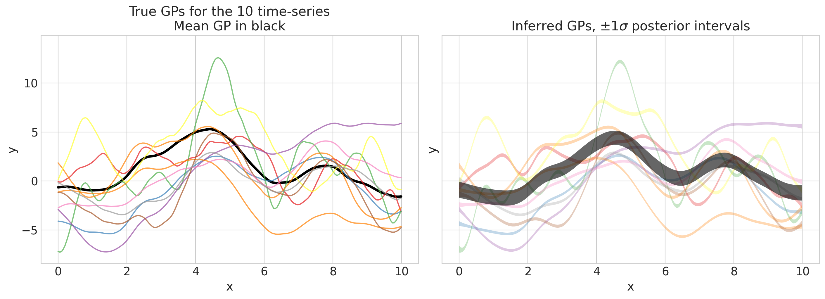
    axs[0].set(ylim=ylims, title="True GPs for the 10 time-series\nMean GP in black")
    axs[1].set(ylim=ylims, title=r"Inferred GPs, $\pm 1 \sigma$ posterior intervals")

    if return_f:
        return f_mu_mu, f_mu_sd, f_mu, f_sd

plot_gps(idata, f_mu_true_train, f_true_train, group="prior");

../../../_images/e6a9dc53ec004ed3519c99b69a90e24733a16a885c756b3de31a36d159d39b37.png

一旦我们对我们的先验感到满意，就像这里的情况一样，我们就可以… 对模型进行采样！

采样与收敛检查#

with model:
    idata.extend(pm.sample(nuts_sampler="numpyro", target_accept=0.9, random_seed=rng))

/home/osvaldo/anaconda3/envs/pymc/lib/python3.11/site-packages/jax/_src/interpreters/mlir.py:790: UserWarning: Some donated buffers were not usable: ShapedArray(float64[4,1000,9]).
See an explanation at https://jax.readthedocs.io/en/latest/faq.html#buffer-donation.
  warnings.warn("Some donated buffers were not usable:"
2024-08-17 10:20:29.439310: E external/xla/xla/service/slow_operation_alarm.cc:65] Constant folding an instruction is taking > 1s:

  %reduce.6 = f64[4,1000,100,10]{3,2,1,0} reduce(f64[4,1000,1,100,10]{4,3,2,1,0} %broadcast.12, f64[] %constant.39), dimensions={2}, to_apply=%region_3.199, metadata={op_name="jit(process_fn)/jit(main)/reduce_prod[axes=(2,)]" source_file="/tmp/tmpzkk5vu9q" source_line=125}

This isn't necessarily a bug; constant-folding is inherently a trade-off between compilation time and speed at runtime. XLA has some guards that attempt to keep constant folding from taking too long, but fundamentally you'll always be able to come up with an input program that takes a long time.

If you'd like to file a bug, run with envvar XLA_FLAGS=--xla_dump_to=/tmp/foo and attach the results.
2024-08-17 10:20:31.621028: E external/xla/xla/service/slow_operation_alarm.cc:133] The operation took 3.185249099s
Constant folding an instruction is taking > 1s:

  %reduce.6 = f64[4,1000,100,10]{3,2,1,0} reduce(f64[4,1000,1,100,10]{4,3,2,1,0} %broadcast.12, f64[] %constant.39), dimensions={2}, to_apply=%region_3.199, metadata={op_name="jit(process_fn)/jit(main)/reduce_prod[axes=(2,)]" source_file="/tmp/tmpzkk5vu9q" source_line=125}

This isn't necessarily a bug; constant-folding is inherently a trade-off between compilation time and speed at runtime. XLA has some guards that attempt to keep constant folding from taking too long, but fundamentally you'll always be able to come up with an input program that takes a long time.

If you'd like to file a bug, run with envvar XLA_FLAGS=--xla_dump_to=/tmp/foo and attach the results.
There were 2 divergences after tuning. Increase `target_accept` or reparameterize.

idata.sample_stats.diverging.sum().data

array(2)

var_names = ["eta_mu", "ell_mu", "eta_delta", "ell_delta", "sigma"]
az.summary(idata, var_names=var_names, round_to=2, filter_vars="regex")

	mean	sd	hdi_3%	hdi_97%	mcse_mean	mcse_sd	ess_bulk	ess_tail	r_hat
ell_delta[0]	0.87	0.12	0.66	1.12	0.00	0.00	1709.41	2585.89	1.0
ell_delta[1]	2.55	0.58	1.54	3.62	0.01	0.01	1683.63	2477.46	1.0
ell_delta[2]	0.52	0.08	0.38	0.66	0.00	0.00	1885.38	2603.51	1.0
ell_delta[3]	2.30	0.37	1.65	3.00	0.01	0.01	2346.83	2554.60	1.0
ell_delta[4]	1.46	0.18	1.12	1.81	0.00	0.00	2650.76	2751.43	1.0
ell_delta[5]	3.12	0.59	2.06	4.18	0.01	0.01	2385.15	2867.07	1.0
ell_delta[6]	0.74	0.09	0.58	0.90	0.00	0.00	2075.16	2813.10	1.0
ell_delta[7]	1.39	0.17	1.05	1.71	0.00	0.00	2740.15	2762.05	1.0
ell_delta[8]	1.92	0.32	1.35	2.52	0.01	0.01	2065.93	2824.22	1.0
ell_delta[9]	2.08	0.42	1.37	2.87	0.01	0.01	1532.88	2489.98	1.0
ell_mu_short	1.60	0.12	1.37	1.82	0.00	0.00	1636.90	2444.40	1.0
ell_mu_trend	8.47	1.88	5.21	11.96	0.02	0.02	6838.61	3243.74	1.0
eta_delta	2.75	0.23	2.33	3.19	0.01	0.00	1990.77	2872.63	1.0
eta_mu_short	1.93	0.42	1.22	2.76	0.01	0.01	2547.80	3187.95	1.0
eta_mu_trend	3.17	0.92	1.61	4.95	0.01	0.01	5913.79	2946.03	1.0
log_ell_delta_offset[0]	-0.90	0.25	-1.35	-0.42	0.01	0.00	2035.33	2871.62	1.0
log_ell_delta_offset[1]	0.92	0.49	0.07	1.82	0.01	0.01	2155.53	2655.70	1.0
log_ell_delta_offset[2]	-1.51	0.36	-2.19	-0.87	0.01	0.01	2251.33	2944.51	1.0
log_ell_delta_offset[3]	0.71	0.37	0.06	1.41	0.01	0.01	2401.93	2603.21	1.0
log_ell_delta_offset[4]	-0.15	0.20	-0.53	0.23	0.00	0.00	2622.45	2654.41	1.0
log_ell_delta_offset[5]	1.43	0.49	0.56	2.34	0.01	0.01	2829.42	3212.54	1.0
log_ell_delta_offset[6]	-1.10	0.28	-1.64	-0.61	0.01	0.00	2061.39	2636.77	1.0
log_ell_delta_offset[7]	-0.22	0.20	-0.61	0.16	0.00	0.00	2662.13	2985.99	1.0
log_ell_delta_offset[8]	0.33	0.32	-0.20	0.94	0.01	0.00	2288.21	2789.51	1.0
log_ell_delta_offset[9]	0.49	0.39	-0.18	1.25	0.01	0.01	1344.83	2505.93	1.0
log_ell_delta_sd	1.23	0.33	0.70	1.85	0.01	0.01	1866.19	2403.58	1.0
log_ell_mu_short	1.37	0.15	1.08	1.64	0.00	0.00	1636.90	2444.40	1.0
sigma	0.52	0.01	0.50	0.53	0.00	0.00	7073.09	2954.36	1.0

ref_val_lines = [
    ("eta_mu_short", {}, [eta_mu_short_true]),
    ("eta_mu_trend", {}, [eta_mu_trend_true]),
    ("ell_mu_short", {}, [ell_mu_short_true]),
    ("ell_mu_trend", {}, [ell_mu_trend_true]),
    ("eta_delta", {}, [eta_delta_true]),
    ("ell_delta", {}, [ell_delta_true]),
    ("sigma", {}, [sigma_noise]),
]

az.plot_trace(
    idata,
    var_names=["eta_mu", "ell_mu", "eta_delta", "ell_delta", "sigma"],
    lines=ref_val_lines,
    filter_vars="regex",
);

../../../_images/a64e90e820d4bc9b934741827ef6d5f4b9cb1016a9ebae448839d9732cd93573.png

一切都很顺利，这真是个好兆头！现在让我们看看模型是否能恢复真实参数。

后验检查#

az.plot_posterior(
    idata,
    var_names=[
        "eta_mu_short",
        "eta_mu_trend",
        "ell_mu_short",
        "ell_mu_trend",
        "eta_delta",
        "ell_delta",
        "sigma",
    ],
    ref_val={
        "eta_mu_short": [{"ref_val": eta_mu_short_true}],
        "eta_mu_trend": [{"ref_val": eta_mu_trend_true}],
        "ell_mu_short": [{"ref_val": ell_mu_short_true}],
        "ell_mu_trend": [{"ref_val": ell_mu_trend_true}],
        "eta_delta": [{"ref_val": eta_delta_true}],
        "ell_delta": [{"gp_ix": i, "ref_val": ell_delta_true[i]} for i in range(n_gps)],
        "sigma": [{"ref_val": sigma_noise}],
    },
    grid=(6, 3),
    textsize=30,
);

../../../_images/31016a9334c34ea8bcf393ab90c56841314c0c49bcdf1038561cea0534921822.png

真的做得很好——模型很好地恢复了所有内容！

az.plot_forest(
    [idata.prior, idata.posterior],
    model_names=["Prior", "Posterior"],
    var_names=[
        "eta_mu_short",
        "eta_mu_trend",
        "ell_mu_short",
        "ell_mu_trend",
        "eta_delta",
        "ell_delta",
        "sigma",
    ],
    combined=True,
    figsize=(12, 6),
);

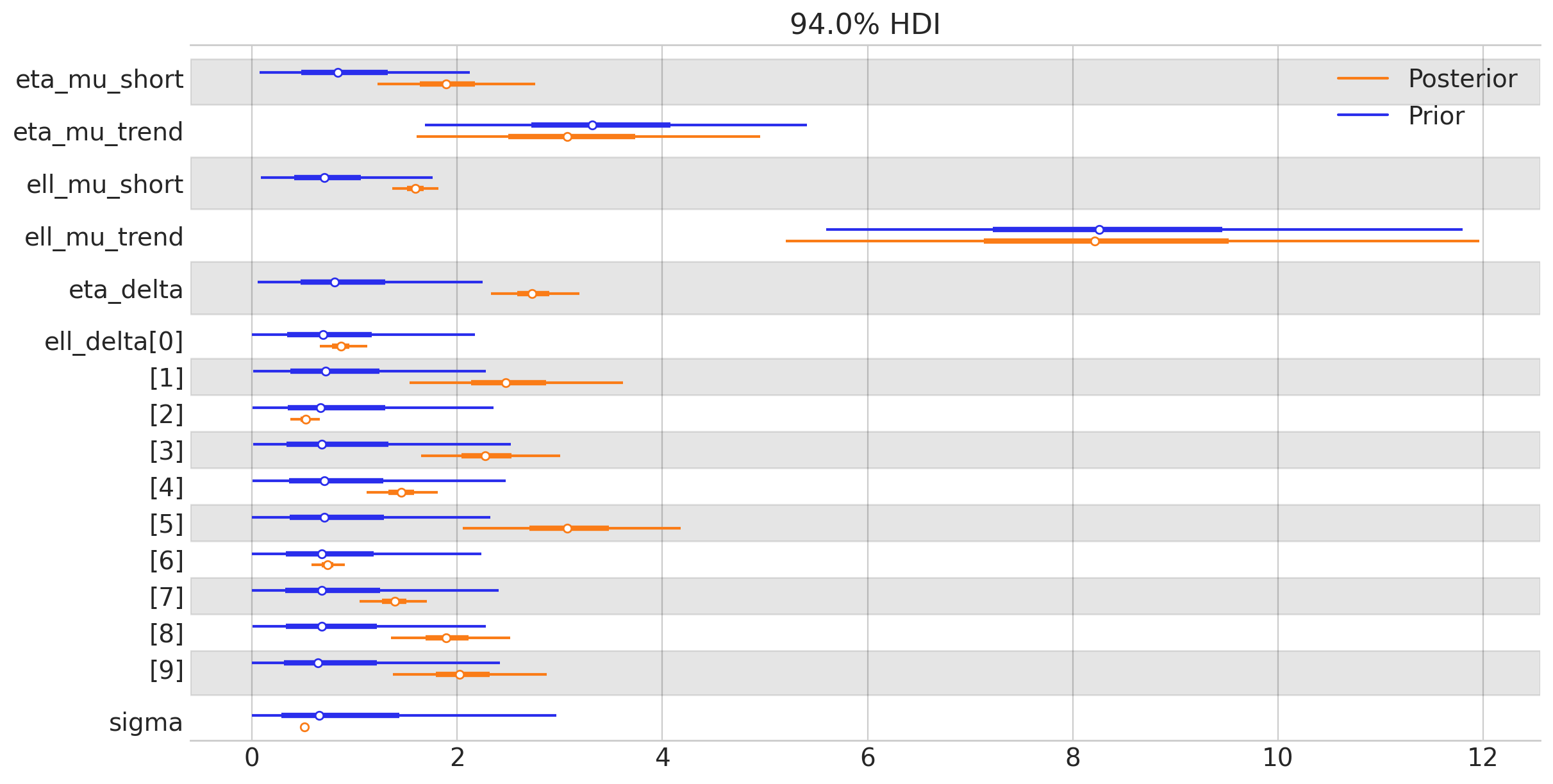
../../../_images/a47bd00cea166277c1c0eb9185759649bbf3eaab74a025726d6626c924c669f5.png

我们可以看到，GP参数很好地被数据所确定。让我们通过用推断出的GP后验更新我们的先验预测图来结束这一部分：

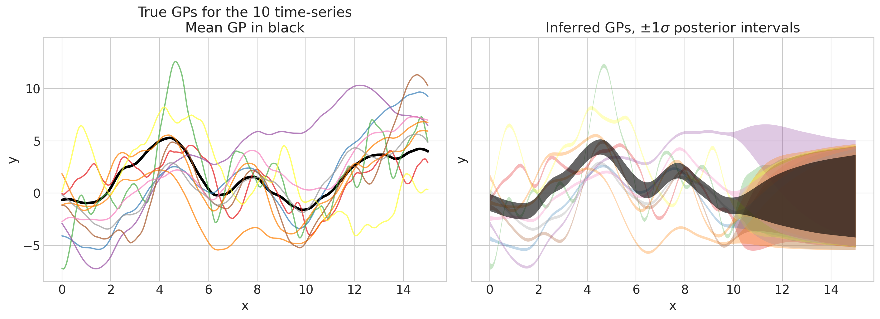
plot_gps(idata, f_mu_true_train, f_true_train);

../../../_images/90f6094e350987d2210f65ea69e47f68e9684e98e9e8b63a9fbe6c432be21065.png

看起来很棒！现在我们可以继续进行样本外预测。

样本外预测#

with model:
    pm.set_data({"X": x_full[:, None]})

    idata.extend(
        pm.sample_posterior_predictive(
            idata,
            var_names=["f_mu", "f"],
            predictions=True,
            compile_kwargs={"mode": "NUMBA"},
            random_seed=rng,
        ),
    )

Sampling: []

pred_f_mu_mu, pred_f_mu_sd, pred_f_mu, pred_f_sd = plot_gps(
    idata, f_mu_true_full, f_true_full, group="predictions", return_f=True
)

../../../_images/e1995fe7492c23e23f28671b77ae6edc1add5d337617b92f78603a57bbd5f4f3.png

这看起来不错！我们可以通过另一个图来检查我们的预测是否合理：

Show code cell source Hide code cell source

fig, axs = plt.subplot_mosaic(
    [["True", "Data"], ["Preds", "Preds"], ["Subset", "Subset"]],
    layout="constrained",
    sharex=True,
    sharey=True,
    figsize=(12, 10),
)

axs["True"].plot(x_train, f_mu_true_train, color="C1", lw=3)
axs["True"].plot(x_test, f_mu_true_test, color="C1", lw=3, ls="--")
axs["True"].axvline(x_train[-1], ls=":", lw=3, color="k", alpha=0.6)
axs["True"].text(
    train_text_x,
    text_y,
    "Training territory",
    horizontalalignment="center",
    verticalalignment="center",
    fontsize=14,
    color="blue",
    alpha=0.7,
)
axs["True"].text(
    test_text_x,
    text_y,
    "Testing territory",
    horizontalalignment="center",
    verticalalignment="center",
    fontsize=14,
    color="green",
    alpha=0.7,
)
axs["Data"].axvline(x_train[-1], ls=":", lw=3, color="k", alpha=0.6)
axs["Preds"].axvline(x_train[-1], ls=":", lw=3, color="k", alpha=0.6)
axs["Subset"].axvline(x_train[-1], ls=":", lw=3, color="k", alpha=0.6)
axs["Preds"].axhline(lw=1, color="k", alpha=0.6)
axs["Subset"].axhline(lw=1, color="k", alpha=0.6)

# Plot mean GP
axs["Preds"].fill_between(
    x_full,
    pred_f_mu_mu - pred_f_mu_sd,
    pred_f_mu_mu + pred_f_mu_sd,
    color="C1",
    alpha=0.8,
    edgecolor="none",
)
axs["Subset"].fill_between(
    x_full,
    pred_f_mu_mu - pred_f_mu_sd,
    pred_f_mu_mu + pred_f_mu_sd,
    color="C1",
    alpha=0.8,
    edgecolor="none",
)
axs["Subset"].plot(
    x_full,
    pred_f_mu_mu,
    color="k",
    alpha=0.5,
    ls="--",
    label="Mean GP",
)

for i in range(n_gps):
    axs["True"].plot(x_train, f_true_train[:, i], color=colors_train[i])
    axs["True"].plot(x_test, f_true_test[:, i], color=colors_test[i])
    axs["Data"].scatter(x_train, y_train[:, i], color=colors_train[i], alpha=0.6)
    axs["Data"].scatter(x_test, y_test[:, i], color=colors_test[i], alpha=0.6)

    # Plot inferred GPs with uncertainty
    axs["Preds"].fill_between(
        x_train,
        pred_f_mu[:n_train, i] - pred_f_sd[:n_train, i],
        pred_f_mu[:n_train, i] + pred_f_sd[:n_train, i],
        color=colors_train[i],
        alpha=0.3,
        edgecolor="none",
    )
    axs["Preds"].fill_between(
        x_test,
        pred_f_mu[n_train:, i] - pred_f_sd[n_train:, i],
        pred_f_mu[n_train:, i] + pred_f_sd[n_train:, i],
        color=colors_test[i],
        alpha=0.3,
        edgecolor="none",
    )

i = rng.choice(n_gps)
axs["Subset"].fill_between(
    x_train,
    pred_f_mu[:n_train, i] - pred_f_sd[:n_train, i],
    pred_f_mu[:n_train, i] + pred_f_sd[:n_train, i],
    color="C0",
    alpha=0.4,
    edgecolor="none",
)
axs["Subset"].fill_between(
    x_test,
    pred_f_mu[n_train:, i] - pred_f_sd[n_train:, i],
    pred_f_mu[n_train:, i] + pred_f_sd[n_train:, i],
    color="C2",
    alpha=0.4,
    edgecolor="none",
)
axs["Subset"].plot(
    x_full,
    pred_f_mu[:, i],
    color="k",
    alpha=0.6,
    ls="-.",
    label="Offset GP",
)

axs["True"].set(xlabel="x", ylim=ylims, title="True GPs\nMean GP in orange")
axs["Data"].set(xlabel="x", ylim=ylims, title="Observed data\nColor corresponding to GP")
axs["Preds"].set(
    xlabel="x",
    ylim=ylims,
    title="Predicted GPs, $\\pm 1 \\sigma$ posterior intervals\nMean GP in orange",
)
axs["Subset"].set(
    xlabel="x",
    ylim=ylims,
    title="Mean GP and Randomly drawn Offset GP",
)
axs["Subset"].legend(title="Average of:", frameon=True, ncols=2, fontsize=10, title_fontsize=11);

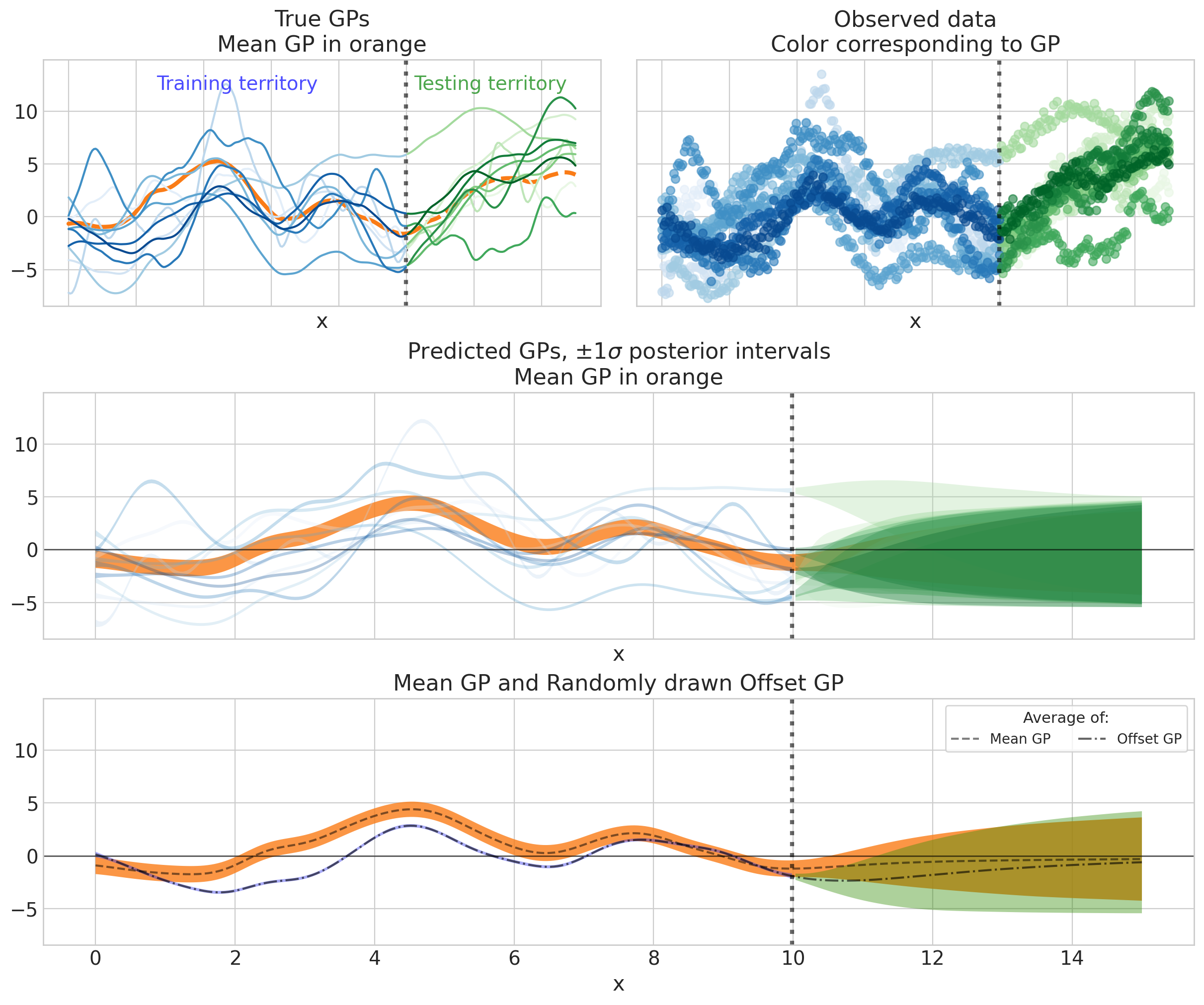
../../../_images/22c69cc6639084ce32012e1c3cc22d9c34a8e1453ffafd91f5016d4ce20803ba.png

哎呀，信息量真大！让我们看看能从中得出什么：

随着数据变得稀疏，长期趋势正在回归到总体GP均值（即0），但尚未达到，因为趋势的长度尺度大于5的测试周期（ell_mu_trend_true = 10）。
由于短期变化相对于趋势较小，平均GP的短期变化并不明显。但它确实是显著的：它导致了橙色HDI中的小波动，并使得这个HDI相对于单个GP（蓝色部分）更宽。
个体GP比回归到GP均值（即0）更快地回归到均值GP（橙色包络线），这是我们希望从层次结构中得到的行为。

示例 2：利用Kronecker结构的HSGP#

这个示例与之前的多个GP模型类似，但它假设了GP之间的不同关系。与向共同均值GP汇聚不同，这里有一个额外的协方差结构来指定它们之间的关系。

例如，我们可能有多家气象站的时间序列温度测量数据。时间上的相似性主要应仅取决于气象站之间的距离。它们在时间上可能具有相同的动态特性或相同的协方差结构。你可以将其视为局部部分池化。

在下面的示例中，我们将GP沿一个“空间”轴排列，因此这是一个1D问题而不是2D问题，然后允许它们共享相同的时间协方差。查看下面的模拟数据后，这可能会更清晰。

在数学上，该模型使用了克罗内克积，其中“空间”和“时间”维度是可分离的。

\[ K = K_{x} \otimes K_{t} \]

如果有\(n_t\)个时间点和\(n_x\)个高斯过程，那么生成的\(K\)矩阵将具有维度\(n_x \cdot n_t \times n_x \cdot n_t\)。使用常规的高斯过程，这将需要\(\mathcal{O}(n_t^3 n_x^3)\)的计算量。因此，通过利用克罗内克结构并使用HSGP近似，我们可以实现相当大的速度提升。并不要求两个维度（在本例中为空间和时间）都使用HSGP近似。可以为“空间”协方差使用普通的高斯过程或诱导点，而在时间维度上使用HSGP近似。在下面的示例中，两者都使用了HSGP近似。

如果您对此部分感兴趣，请参考：

看到利用Kronecker结构和HSGP近似的示例。
了解如何构建更高级和自定义的GP模型。

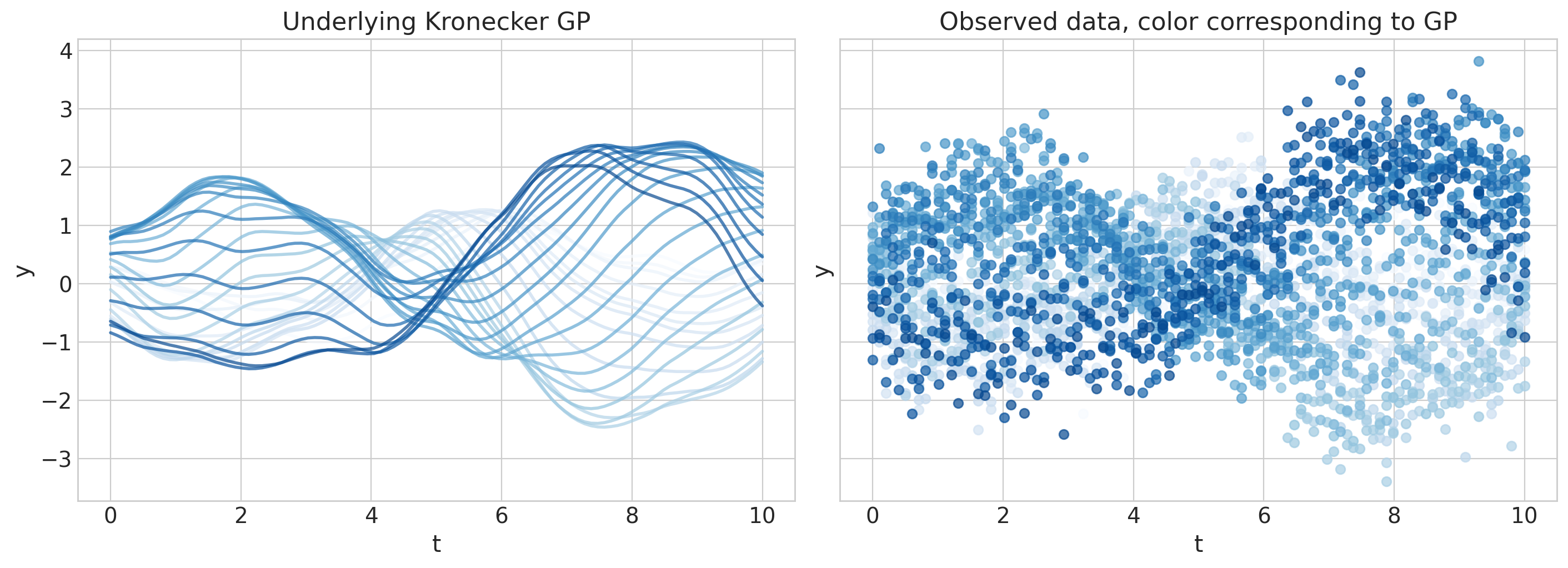
数据生成#

n_gps, n_t = 30, 100
t = np.linspace(0, 10, n_t)
x = np.linspace(-5, 5, n_gps)

eta_true = 1.0
ell_x_true = 2.0
cov_x = eta_true**2 * pm.gp.cov.Matern52(input_dim=1, ls=ell_x_true)
Kx = cov_x(x[:, None])

ell_t_true = 2.0
cov_t = pm.gp.cov.Matern52(input_dim=1, ls=ell_t_true)
Kt = cov_t(t[:, None])

K = pt.slinalg.kron(Kx, Kt)
f_true = (
    pm.draw(pm.MvNormal.dist(mu=np.zeros(n_gps * n_t), cov=K), random_seed=rng)
    .reshape(n_gps, n_t)
    .T
)

# Additive gaussian noise
sigma_noise = 0.5
noise_dist = pm.Normal.dist(mu=0.0, sigma=sigma_noise)

y_obs = f_true + pm.draw(noise_dist, draws=n_t * n_gps, random_seed=rng).reshape(n_t, n_gps)

fig, axs = plt.subplots(1, 2, figsize=(14, 5), sharex=True, sharey=True)
colors = plt.cm.Blues(np.linspace(0.0, 0.9, n_gps))
ylims = [1.1 * np.min(y_obs), 1.1 * np.max(y_obs)]

for i in range(n_gps):
    axs[0].plot(t, f_true[:, i], color=colors[i], lw=2, alpha=0.7)
    axs[1].scatter(t, y_obs[:, i], color=colors[i], alpha=0.7)

for ax in axs:
    ax.set_xlabel("t")
    ax.set_ylabel("y")
axs[0].set(ylim=ylims, title="Underlying Kronecker GP")
axs[1].set(ylim=ylims, title="Observed data, color corresponding to GP");

../../../_images/23caeed7626c7739ce78580034bb358083fbe9b0edd30977166cafce36da55ce.png

Kronecker GP 规范#

def kronecker_HSGP(Xs, m, c, cov_t, cov_x):
    Xs_t, Xs_x = Xs  # Xs needs to be 0-centered
    m_t, m_x = m
    c_t, c_x = c

    L_t = pm.gp.hsgp_approx.set_boundary(Xs_t, c_t)
    eigvals_t = pm.gp.hsgp_approx.calc_eigenvalues(L_t, [m_t])
    phi_t = pm.gp.hsgp_approx.calc_eigenvectors(Xs_t, L_t, eigvals_t, [m_t])
    omega_t = pt.sqrt(eigvals_t)

    sqrt_psd_t = pt.sqrt(cov_t.power_spectral_density(omega_t))
    chol_t = phi_t * sqrt_psd_t

    L_x = pm.gp.hsgp_approx.set_boundary(Xs_x, c_x)
    eigvals_x = pm.gp.hsgp_approx.calc_eigenvalues(L_x, [m_x])
    phi_x = pm.gp.hsgp_approx.calc_eigenvectors(Xs_x, L_x, eigvals_x, [m_x])
    omega_x = pt.sqrt(eigvals_x)

    sqrt_psd_x = pt.sqrt(cov_x.power_spectral_density(omega_x))
    chol_x = phi_x * sqrt_psd_x

    z = pm.Normal("beta", size=m_x * m_t)

    return (chol_x @ (chol_t @ pt.reshape(z, (m_t, m_x))).T).T

PyMC 模型#

接下来，我们使用启发式方法来选择 m 和 c：

m_t, c_t = pm.gp.hsgp_approx.approx_hsgp_hyperparams(
    x_range=[np.min(t), np.max(t)], lengthscale_range=[1.0, 3.0], cov_func="matern52"
)
m_x, c_x = pm.gp.hsgp_approx.approx_hsgp_hyperparams(
    x_range=[np.min(x), np.max(x)], lengthscale_range=[1.0, 3.0], cov_func="matern52"
)

print(f"m_t: {m_t}, c_t: {c_t:.2f}")
print(f"m_x: {m_x}, c_x: {c_x:.2f}")

m_t: 32, c_t: 2.46
m_x: 32, c_x: 2.46

with pm.Model() as model:
    ## handle 0-centering correctly
    xt_center = (np.max(t) + np.min(t)) / 2
    Xt = pm.Data("Xt", t[:, None])
    Xs_t = Xt - xt_center

    xx_center = (np.max(x) + np.min(x)) / 2
    Xx = pm.Data("Xx", x[:, None])
    Xs_x = Xx - xx_center

    ## covariance on time GP
    ell_t = pz.maxent(pz.LogNormal(), lower=0.5, upper=4.0, mass=0.95, plot=False).to_pymc("ell_t")
    cov_t = pm.gp.cov.Matern52(1, ls=ell_t)

    ## covariance on space GP
    ell_x = pz.maxent(pz.LogNormal(), lower=0.5, upper=4.0, mass=0.95, plot=False).to_pymc("ell_x")
    cov_x = pm.gp.cov.Matern52(1, ls=ell_x)

    ## Kronecker GP
    eta = pm.Gamma("eta", 2, 2)
    Xs, m, c = [Xs_t, Xs_x], [m_t, m_x], [c_t, c_x]
    f = kronecker_HSGP(Xs, m, c, cov_t, cov_x)
    f = pm.Deterministic("f", eta * f)

    # observational noise
    sigma = pm.Exponential("sigma", scale=1)

    # likelihood
    pm.Normal("y", mu=f, sigma=sigma, observed=y_obs)

pm.model_to_graphviz(model)

../../../_images/e7ac5484fd8d3a389ec075759fd92759a768acdce6ada061db756b7cce9a079a.svg

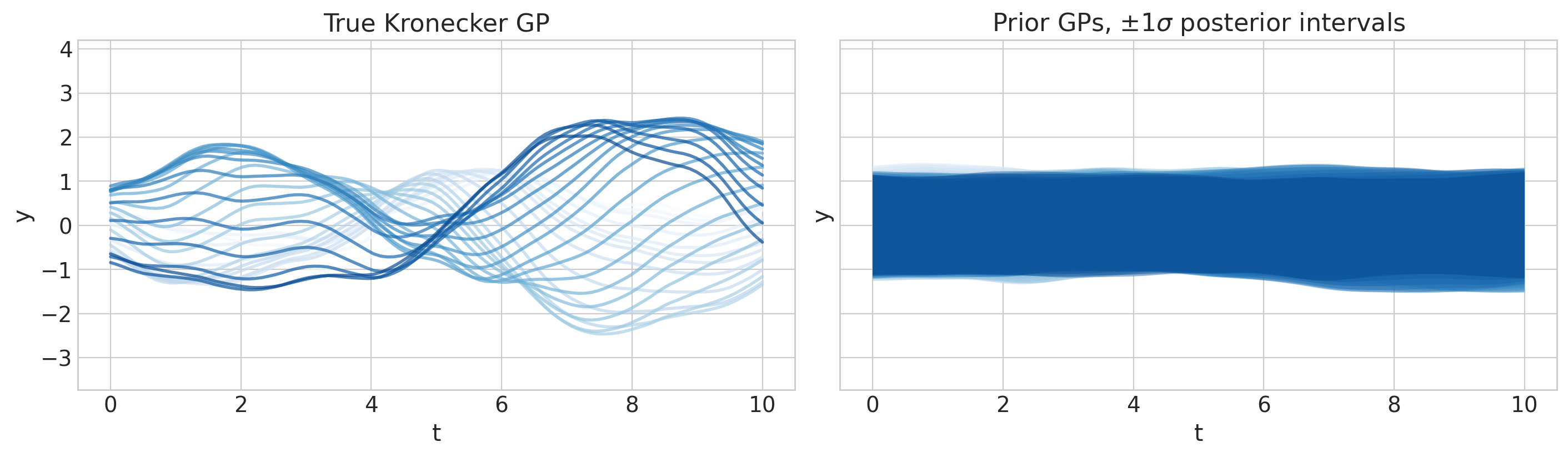
先验预测检查#

with model:
    idata = pm.sample_prior_predictive(random_seed=rng)

Sampling: [beta, ell_t, ell_x, eta, sigma, y]

f_mu = az.extract(idata, group="prior", var_names="f").mean(dim="sample")
f_sd = az.extract(idata, group="prior", var_names="f").std(dim="sample")

fig, axs = plt.subplots(1, 2, figsize=(14, 4), sharex=True, sharey=True)
colors = plt.cm.Blues(np.linspace(0.0, 0.9, n_gps))
ylims = [1.1 * np.min(y_obs), 1.1 * np.max(y_obs)]

for i in range(n_gps):
    axs[0].plot(t, f_true[:, i], color=colors[i], lw=2, alpha=0.7)
    axs[1].fill_between(
        t,
        f_mu[:, i] - f_sd[:, i],
        f_mu[:, i] + f_sd[:, i],
        color=colors[i],
        alpha=0.4,
        edgecolor="none",
    )

for ax in axs:
    ax.set_xlabel("t")
    ax.set_ylabel("y")

axs[0].set(ylim=ylims, title="True Kronecker GP")
axs[1].set(ylim=ylims, title=r"Prior GPs, $\pm 1 \sigma$ posterior intervals");

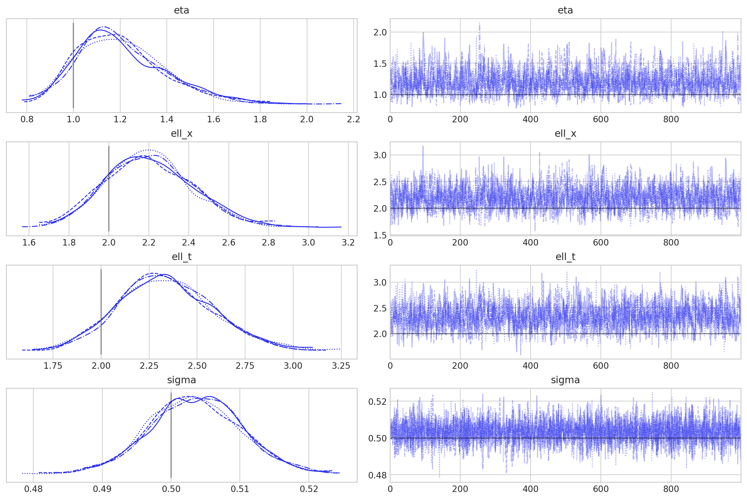
../../../_images/f40c215169f13879d2f85a4623b5746159ed70c351bf51f4e7a05a77e1edbd23.png

采样与收敛检查#

with model:
    idata.extend(pm.sample(nuts_sampler="numpyro", random_seed=rng))

2024-08-17 10:22:58.363258: E external/xla/xla/service/slow_operation_alarm.cc:65] Constant folding an instruction is taking > 2s:

  %reduce.3 = f64[4,1000,100,32]{3,2,1,0} reduce(f64[4,1000,1,100,32]{4,3,2,1,0} %broadcast.7, f64[] %constant.24), dimensions={2}, to_apply=%region_3.90, metadata={op_name="jit(process_fn)/jit(main)/reduce_prod[axes=(2,)]" source_file="/tmp/tmp2qa9axab" source_line=55}

This isn't necessarily a bug; constant-folding is inherently a trade-off between compilation time and speed at runtime. XLA has some guards that attempt to keep constant folding from taking too long, but fundamentally you'll always be able to come up with an input program that takes a long time.

If you'd like to file a bug, run with envvar XLA_FLAGS=--xla_dump_to=/tmp/foo and attach the results.
2024-08-17 10:23:10.111194: E external/xla/xla/service/slow_operation_alarm.cc:133] The operation took 13.753874175s
Constant folding an instruction is taking > 2s:

  %reduce.3 = f64[4,1000,100,32]{3,2,1,0} reduce(f64[4,1000,1,100,32]{4,3,2,1,0} %broadcast.7, f64[] %constant.24), dimensions={2}, to_apply=%region_3.90, metadata={op_name="jit(process_fn)/jit(main)/reduce_prod[axes=(2,)]" source_file="/tmp/tmp2qa9axab" source_line=55}

This isn't necessarily a bug; constant-folding is inherently a trade-off between compilation time and speed at runtime. XLA has some guards that attempt to keep constant folding from taking too long, but fundamentally you'll always be able to come up with an input program that takes a long time.

If you'd like to file a bug, run with envvar XLA_FLAGS=--xla_dump_to=/tmp/foo and attach the results.
2024-08-17 10:23:14.126717: E external/xla/xla/service/slow_operation_alarm.cc:65] Constant folding an instruction is taking > 4s:

  %reduce.4 = f64[4,1000,100,32]{3,2,1,0} reduce(f64[4,1000,1,100,32]{4,3,2,1,0} %broadcast.88, f64[] %constant.24), dimensions={2}, to_apply=%region_3.90, metadata={op_name="jit(process_fn)/jit(main)/reduce_prod[axes=(2,)]" source_file="/tmp/tmp2qa9axab" source_line=55}

This isn't necessarily a bug; constant-folding is inherently a trade-off between compilation time and speed at runtime. XLA has some guards that attempt to keep constant folding from taking too long, but fundamentally you'll always be able to come up with an input program that takes a long time.

If you'd like to file a bug, run with envvar XLA_FLAGS=--xla_dump_to=/tmp/foo and attach the results.
2024-08-17 10:23:23.419691: E external/xla/xla/service/slow_operation_alarm.cc:133] The operation took 13.293039547s
Constant folding an instruction is taking > 4s:

  %reduce.4 = f64[4,1000,100,32]{3,2,1,0} reduce(f64[4,1000,1,100,32]{4,3,2,1,0} %broadcast.88, f64[] %constant.24), dimensions={2}, to_apply=%region_3.90, metadata={op_name="jit(process_fn)/jit(main)/reduce_prod[axes=(2,)]" source_file="/tmp/tmp2qa9axab" source_line=55}

This isn't necessarily a bug; constant-folding is inherently a trade-off between compilation time and speed at runtime. XLA has some guards that attempt to keep constant folding from taking too long, but fundamentally you'll always be able to come up with an input program that takes a long time.

If you'd like to file a bug, run with envvar XLA_FLAGS=--xla_dump_to=/tmp/foo and attach the results.
2024-08-17 10:23:31.419862: E external/xla/xla/service/slow_operation_alarm.cc:65] Constant folding an instruction is taking > 8s:

  %map.2 = f64[4,1000,100,32]{3,2,1,0} map(f64[4,1000,100,32]{3,2,1,0} %constant, f64[4,1000,100,32]{3,2,1,0} %constant.2), dimensions={0,1,2,3}, to_apply=%region_3.90, metadata={op_name="jit(process_fn)/jit(main)/reduce_prod[axes=(2,)]" source_file="/tmp/tmp2qa9axab" source_line=55}

This isn't necessarily a bug; constant-folding is inherently a trade-off between compilation time and speed at runtime. XLA has some guards that attempt to keep constant folding from taking too long, but fundamentally you'll always be able to come up with an input program that takes a long time.

If you'd like to file a bug, run with envvar XLA_FLAGS=--xla_dump_to=/tmp/foo and attach the results.
2024-08-17 10:23:50.806267: E external/xla/xla/service/slow_operation_alarm.cc:133] The operation took 27.386498208s
Constant folding an instruction is taking > 8s:

  %map.2 = f64[4,1000,100,32]{3,2,1,0} map(f64[4,1000,100,32]{3,2,1,0} %constant, f64[4,1000,100,32]{3,2,1,0} %constant.2), dimensions={0,1,2,3}, to_apply=%region_3.90, metadata={op_name="jit(process_fn)/jit(main)/reduce_prod[axes=(2,)]" source_file="/tmp/tmp2qa9axab" source_line=55}

This isn't necessarily a bug; constant-folding is inherently a trade-off between compilation time and speed at runtime. XLA has some guards that attempt to keep constant folding from taking too long, but fundamentally you'll always be able to come up with an input program that takes a long time.

If you'd like to file a bug, run with envvar XLA_FLAGS=--xla_dump_to=/tmp/foo and attach the results.

idata.sample_stats.diverging.sum().data

array(0)

az.summary(idata, var_names=["eta", "ell_x", "ell_t", "sigma"], round_to=2)

	mean	sd	hdi_3%	hdi_97%	mcse_mean	ess_bulk	ess_tail	r_hat
eta	1.21	0.19	0.88	1.58	0.00	1549.16	2142.20	1.0
ell_x	2.21	0.22	1.82	2.62	0.01	1668.86	2593.89	1.0
ell_t	2.34	0.24	1.89	2.81	0.01	1606.45	2366.53	1.0
sigma	0.50	0.01	0.49	0.52	0.00	6315.09	2993.34	1.0

az.plot_trace(
    idata,
    var_names=["eta", "ell_x", "ell_t", "sigma"],
    lines=[
        ("eta", {}, [eta_true]),
        ("ell_x", {}, [ell_x_true]),
        ("ell_t", {}, [ell_t_true]),
        ("sigma", {}, [sigma_noise]),
    ],
);

../../../_images/e5edc7c2a05b17f92f574c38cbd767d5ba0bbadee7b4512874e8827fe01060aa.png

后验预测检查#

f_mu = az.extract(idata, group="posterior", var_names="f").mean(dim="sample")
f_sd = az.extract(idata, group="posterior", var_names="f").std(dim="sample")

fig, axs = plt.subplots(1, 2, figsize=(14, 5), sharex=True, sharey=True)
colors = plt.cm.Blues(np.linspace(0.0, 0.9, n_gps))
ylims = [1.1 * np.min(y_obs), 1.1 * np.max(y_obs)]

for i in range(n_gps):
    axs[0].plot(t, f_true[:, i], color=colors[i], lw=2, alpha=0.7)
    axs[1].fill_between(
        t,
        f_mu[:, i] - f_sd[:, i],
        f_mu[:, i] + f_sd[:, i],
        color=colors[i],
        alpha=0.4,
        edgecolor="none",
    )

for ax in axs:
    ax.set_xlabel("t")
    ax.set_ylabel("y")

axs[0].set(ylim=ylims, title="True Kronecker GP")
axs[1].set(ylim=ylims, title=r"Prior GPs, $\pm 1 \sigma$ posterior intervals");

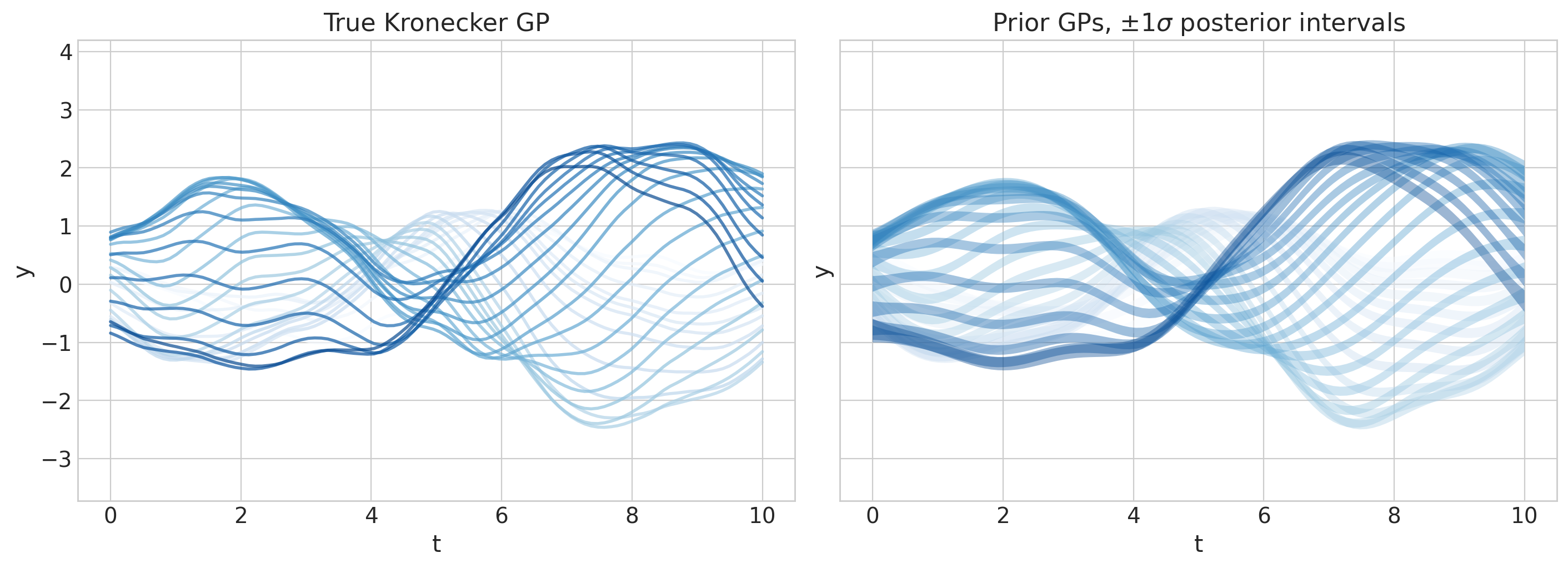
../../../_images/81cf6b9105f7b112fec1d2fa2c5a5025d6fbde203363de5f422336750f8340de.png

这不是很美吗？现在继续，并HSGP-on！

作者#

由 Bill Engels、Alexandre Andorra 和 Maxim Kochurov 于2024年创建（pymc-examples#668）
使用 pz.maxent 代替 pm.find_constrained_prior，并添加随机种子。Osvaldo Martin。2024年8月

水印#

%load_ext watermark
%watermark -n -u -v -iv -w -p xarray

Last updated: Sat Aug 17 2024

Python implementation: CPython
Python version       : 3.11.5
IPython version      : 8.16.1

xarray: 2023.10.1

arviz     : 0.19.0.dev0
preliz    : 0.9.0
pymc      : 5.16.2+20.g747fda319
numpy     : 1.24.4
pytensor  : 2.25.2
matplotlib: 3.8.4

Watermark: 2.4.3

分类

标签

高斯过程：HSGP 高级用法#

参考资料：#

示例 1：一个分层的 HSGP，一个更自定义的模型#

模拟数据#

定义均值GP#

分层建模的Delta GPs#

辅助函数#

为完整数据生成样本#

可视化生成的数据#

构建模型#

适应功率谱密度#

编码层次化GP#

选择HSGP参数#

设置模型#

先验预测检查#

采样与收敛检查#

后验检查#

样本外预测#

示例 2：利用Kronecker结构的HSGP#

数据生成#

Kronecker GP 规范#

PyMC 模型#

先验预测检查#

采样与收敛检查#

后验预测检查#

作者#

水印#