


离散选择与随机效用模型#
import arviz as az
import numpy as np  # For vectorized math operations
import pandas as pd  # For file input/output
import pymc as pm
import pytensor.tensor as pt

from matplotlib import pyplot as plt
from matplotlib.lines import Line2D
%config InlineBackend.figure_format = 'retina'  # high resolution figures
az.style.use("arviz-darkgrid")
rng = np.random.default_rng(42)
离散选择建模:概念#
离散选择模型与潜在效用尺度的概念有关,如在有序分类结果的回归模型中所讨论的,但它将这一概念推广到决策制定中。它假设人类决策可以被建模为一组互斥备选方案上的潜在/主观效用测量的函数。该理论指出,任何决策者都会选择最大化其主观效用的选项,并且该效用可以被建模为世界可观察特征的潜在线性函数。
这一想法或许最著名地由丹尼尔·麦克法登在20世纪70年代应用于预测加州在提议引入BART轻轨系统后,交通选择(即汽车、铁路、步行等)所占的市场份额。值得在此停顿一下。该理论是关于微观层面的人类决策制定,在实际应用中,已被扩展到做出广泛准确的宏观层面预测。更多详情,我们推荐Train [2009]
我们也不需要过于轻信。这仅仅是一个统计模型,这里的成功完全取决于建模者的技能、可用的测量数据以及合理的理论。但值得注意的是这些模型背后所蕴含的雄心壮志。模型的结构鼓励你阐述你对决策者及其所处环境的理论。
数据#
在这个例子中,我们将研究使用离散选择建模技术,使用来自R mlogit 包的(i) 供暖系统数据集和(ii) 饼干品牌的重复选择数据集。我们将采用贝叶斯方法来估计模型,而不是他们vigenette中报告的MLE方法。第一个数据集显示了加州家庭在供暖系统优惠上的选择。观察结果包括加州新建的单户住宅,这些住宅配有中央空调。考虑了五种可能的系统类型:
燃气中央(gc),
气体室 (gr),
电力中心 (ec),
电气室 (ER),
热泵 (hp)。
数据集报告了每个家庭在五种选择中面临的安装成本 ic.alt 和运营成本 oc.alt,以及一些关于家庭的基本人口信息,最重要的是选择 depvar。以下是数据中五种选择中的一种选择场景的示例:
try:
    wide_heating_df = pd.read_csv("../data/heating_data_r.csv")
except:
    wide_heating_df = pd.read_csv(pm.get_data("heating_data_r.csv"))

wide_heating_df[wide_heating_df["idcase"] == 1]
| idcase | depvar | ic.gc | ic.gr | ic.ec | ic.er | ic.hp | oc.gc | oc.gr | oc.ec | oc.er | oc.hp | income | agehed | rooms | region | |
|---|---|---|---|---|---|---|---|---|---|---|---|---|---|---|---|---|
| 0 | 1 | gc | 866.0 | 962.64 | 859.9 | 995.76 | 1135.5 | 199.69 | 151.72 | 553.34 | 505.6 | 237.88 | 7 | 25 | 6 | ncostl |
这类模型的核心思想是将这种情况视为在具有潜在效用的详尽选项中进行选择。分配给每个选项的效用被视为每个选项属性的线性组合。分配给每个替代方案的效用驱动了在每个选项中选择的概率。对于所有替代方案 \(Alt = \{ gc, gr, ec, er, hp \}\) 中的每个 \(j\),假设其服从Gumbel分布,因为这具有特别好的数学性质。
这一假设在数学上证明是方便的,因为两个Gumbel分布之间的差异可以被建模为一个logistic函数,这意味着我们可以使用softmax函数来建模多个选项之间的对比差异。推导的详细信息可以在Train [2009]中找到
然后,模型假设决策者选择最大化其主观效用的选项。个体效用函数可以进行丰富的参数化。当备选方案的效用度量与“外部商品”的固定效用进行基准比较时,模型就被识别出来。最后一个量固定为0。
在应用了所有这些约束条件后,我们可以构建条件随机效用模型及其层次变体。与统计学中的几乎所有主题一样,模型规范的精确词汇是多义的。条件逻辑回归参数 \(\beta\)
可以在个体层面固定,但也可以在个体和备选方案之间变化 gc, gr, ec, er。通过这种方式,我们可以构建一个复杂的理论,说明我们预期主观效用的驱动因素如何改变一组竞争商品的市场份额。
关于数据格式的题外话#
离散选择模型通常使用长数据格式进行估计,其中每个选择场景由每个替代ID的一行和一个二进制标志表示,该标志表示每个场景中选择的选项。建议在stan和pylogit中估计这类模型时使用这种数据格式。这样做的原因是,一旦installation_costs和operating_costs列以这种方式进行透视,将它们包含在矩阵计算中会更容易。
try:
    long_heating_df = pd.read_csv("../data/long_heating_data.csv")
except:
    long_heating_df = pd.read_csv(pm.get_data("long_heating_data.csv"))

columns = [c for c in long_heating_df.columns if c != "Unnamed: 0"]
long_heating_df[long_heating_df["idcase"] == 1][columns]
| idcase | alt_id | choice | depvar | income | agehed | rooms | region | installation_costs | operating_costs | |
|---|---|---|---|---|---|---|---|---|---|---|
| 0 | 1 | 1 | 1 | gc | 7 | 25 | 6 | ncostl | 866.00 | 199.69 |
| 1 | 1 | 2 | 0 | gc | 7 | 25 | 6 | ncostl | 962.64 | 151.72 |
| 2 | 1 | 3 | 0 | gc | 7 | 25 | 6 | ncostl | 859.90 | 553.34 |
| 3 | 1 | 4 | 0 | gc | 7 | 25 | 6 | ncostl | 995.76 | 505.60 |
| 4 | 1 | 5 | 0 | gc | 7 | 25 | 6 | ncostl | 1135.50 | 237.88 |
基本模型#
我们将在这里展示如何在PyMC中结合效用规范。PyMC是一个很好的接口,适用于这种建模,因为它可以非常清晰地表达模型,遵循该方程组的自然数学表达。在这个简单的模型中,你可以看到我们如何分别构建每个备选方案的效用度量方程,然后将它们堆叠在一起,创建我们softmax变换的输入矩阵。
N = wide_heating_df.shape[0]
observed = pd.Categorical(wide_heating_df["depvar"]).codes
coords = {
    "alts_probs": ["ec", "er", "gc", "gr", "hp"],
    "obs": range(N),
}

with pm.Model(coords=coords) as model_1:
    beta_ic = pm.Normal("beta_ic", 0, 1)
    beta_oc = pm.Normal("beta_oc", 0, 1)

    ## Construct Utility matrix and Pivot
    u0 = beta_ic * wide_heating_df["ic.ec"] + beta_oc * wide_heating_df["oc.ec"]
    u1 = beta_ic * wide_heating_df["ic.er"] + beta_oc * wide_heating_df["oc.er"]
    u2 = beta_ic * wide_heating_df["ic.gc"] + beta_oc * wide_heating_df["oc.gc"]
    u3 = beta_ic * wide_heating_df["ic.gr"] + beta_oc * wide_heating_df["oc.gr"]
    u4 = np.zeros(N)  # Outside Good
    s = pm.math.stack([u0, u1, u2, u3, u4]).T

    ## Apply Softmax Transform
    p_ = pm.Deterministic("p", pm.math.softmax(s, axis=1), dims=("obs", "alts_probs"))

    ## Likelihood
    choice_obs = pm.Categorical("y_cat", p=p_, observed=observed, dims="obs")

    idata_m1 = pm.sample_prior_predictive()
    idata_m1.extend(
        pm.sample(nuts_sampler="numpyro", idata_kwargs={"log_likelihood": True}, random_seed=101)
    )
    idata_m1.extend(pm.sample_posterior_predictive(idata_m1))

pm.model_to_graphviz(model_1)
Sampling: [beta_ic, beta_oc, y_cat]
/Users/nathanielforde/mambaforge/envs/pymc_examples_new/lib/python3.9/site-packages/pymc/sampling/mcmc.py:243: UserWarning: Use of external NUTS sampler is still experimental
  warnings.warn("Use of external NUTS sampler is still experimental", UserWarning)
Compiling...
Compilation time =  0:00:01.199248
Sampling...
Sampling time =  0:00:02.165671
Transforming variables...
Transformation time =  0:00:00.404064
Computing Log Likelihood...

idata_m1
-
<xarray.Dataset> Dimensions: (chain: 4, draw: 1000, obs: 900, alts_probs: 5) Coordinates: * chain (chain) int64 0 1 2 3 * draw (draw) int64 0 1 2 3 4 5 6 7 ... 992 993 994 995 996 997 998 999 * obs (obs) int64 0 1 2 3 4 5 6 7 ... 892 893 894 895 896 897 898 899 * alts_probs (alts_probs) <U2 'ec' 'er' 'gc' 'gr' 'hp' Data variables: beta_ic (chain, draw) float64 0.001854 0.001794 ... 0.002087 0.001928 beta_oc (chain, draw) float64 -0.003802 -0.003846 ... -0.00447 -0.004533 p (chain, draw, obs, alts_probs) float64 0.07322 0.1129 ... 0.1111 Attributes: created_at: 2023-07-13T17:29:12.988497 arviz_version: 0.15.1 -
<xarray.Dataset> Dimensions: (chain: 4, draw: 1000, obs: 900) Coordinates: * chain (chain) int64 0 1 2 3 * draw (draw) int64 0 1 2 3 4 5 6 7 8 ... 992 993 994 995 996 997 998 999 * obs (obs) int64 0 1 2 3 4 5 6 7 8 ... 892 893 894 895 896 897 898 899 Data variables: y_cat (chain, draw, obs) int64 4 3 4 2 2 1 1 2 4 1 ... 4 3 2 1 4 2 1 1 0 Attributes: created_at: 2023-07-13T17:29:19.656809 arviz_version: 0.15.1 inference_library: pymc inference_library_version: 5.3.0 -
<xarray.Dataset> Dimensions: (chain: 4, draw: 1000, y_cat_dim_0: 1, y_cat_dim_1: 900) Coordinates: * chain (chain) int64 0 1 2 3 * draw (draw) int64 0 1 2 3 4 5 6 7 ... 993 994 995 996 997 998 999 * y_cat_dim_0 (y_cat_dim_0) int64 0 * y_cat_dim_1 (y_cat_dim_1) int64 0 1 2 3 4 5 6 ... 894 895 896 897 898 899 Data variables: y_cat (chain, draw, y_cat_dim_0, y_cat_dim_1) float64 -1.258 ... -... Attributes: created_at: 2023-07-13T17:29:12.992158 arviz_version: 0.15.1 -
<xarray.Dataset> Dimensions: (chain: 4, draw: 1000) Coordinates: * chain (chain) int64 0 1 2 3 * draw (draw) int64 0 1 2 3 4 5 6 ... 993 994 995 996 997 998 999 Data variables: acceptance_rate (chain, draw) float64 0.9667 1.0 0.8868 ... 0.8931 0.9283 step_size (chain, draw) float64 0.02965 0.02965 ... 0.03209 0.03209 diverging (chain, draw) bool False False False ... False False False energy (chain, draw) float64 1.311e+03 1.311e+03 ... 1.312e+03 n_steps (chain, draw) int64 3 3 3 3 1 11 3 7 3 ... 7 7 7 11 7 3 7 3 tree_depth (chain, draw) int64 2 2 2 2 1 4 2 3 2 ... 2 3 3 3 4 3 2 3 2 lp (chain, draw) float64 1.311e+03 1.311e+03 ... 1.311e+03 Attributes: created_at: 2023-07-13T17:29:12.990891 arviz_version: 0.15.1 -
<xarray.Dataset> Dimensions: (chain: 1, draw: 500, obs: 900, alts_probs: 5) Coordinates: * chain (chain) int64 0 * draw (draw) int64 0 1 2 3 4 5 6 7 ... 492 493 494 495 496 497 498 499 * obs (obs) int64 0 1 2 3 4 5 6 7 ... 892 893 894 895 896 897 898 899 * alts_probs (alts_probs) <U2 'ec' 'er' 'gc' 'gr' 'hp' Data variables: beta_oc (chain, draw) float64 0.05221 0.1678 0.7865 ... 0.5232 -0.09242 p (chain, draw, obs, alts_probs) float64 4.778e-201 ... 4.831e-91 beta_ic (chain, draw) float64 -0.57 -0.8283 0.2129 ... 1.097 0.2006 Attributes: created_at: 2023-07-13T17:29:07.842667 arviz_version: 0.15.1 inference_library: pymc inference_library_version: 5.3.0 -
<xarray.Dataset> Dimensions: (chain: 1, draw: 500, obs: 900) Coordinates: * chain (chain) int64 0 * draw (draw) int64 0 1 2 3 4 5 6 7 8 ... 492 493 494 495 496 497 498 499 * obs (obs) int64 0 1 2 3 4 5 6 7 8 ... 892 893 894 895 896 897 898 899 Data variables: y_cat (chain, draw, obs) int64 4 4 4 4 4 4 4 4 4 4 ... 3 1 1 3 3 3 3 3 3 Attributes: created_at: 2023-07-13T17:29:07.844409 arviz_version: 0.15.1 inference_library: pymc inference_library_version: 5.3.0 -
<xarray.Dataset>
Dimensions:  (obs: 900)
Coordinates:
  * obs      (obs) int64 0 1 2 3 4 5 6 7 8 ... 892 893 894 895 896 897 898 899
Data variables:
    y_cat    (obs) int64 2 2 2 1 1 2 2 2 2 2 2 2 2 ... 2 2 2 2 2 2 2 1 2 2 2 2 2
Attributes:
    created_at:                 2023-07-13T17:29:07.844758
    arviz_version:              0.15.1
    inference_library:          pymc
    inference_library_version:  5.3.0
summaries = az.summary(idata_m1, var_names=["beta_ic", "beta_oc"])
summaries
| mean | sd | hdi_3% | hdi_97% | mcse_mean | mcse_sd | ess_bulk | ess_tail | r_hat | |
|---|---|---|---|---|---|---|---|---|---|
| beta_ic | 0.002 | 0.0 | 0.002 | 0.002 | 0.0 | 0.0 | 1870.0 | 1999.0 | 1.0 |
| beta_oc | -0.004 | 0.0 | -0.005 | -0.004 | 0.0 | 0.0 | 881.0 | 1105.0 | 1.0 |
在mlogit指南中,他们报告了上述模型规范如何导致参数估计不足。他们指出,例如,尽管效用尺度本身难以解释,但系数比值通常是有意义的,因为当:
那么边际替代率就是两个beta系数的比率。即使主观效用的概念本身是不可观察的,效用方程中一个组成部分相对于另一个组成部分的相对重要性在经济上也是一个有意义的量。
我们的参数估计与报告的估计略有不同,但我们同意该模型是不充分的。我们将展示一系列贝叶斯模型检查来证明这一事实,但主要需要注意的是安装成本的参数值可能应该是负的。价格增加\(\beta_{ic}\)反而会略微增加安装带来的效用,这似乎是违反直觉的。尽管我们可能会想象到价格带来的某种质量保证会随着安装成本的增加而提高满意度。重复运营成本的系数如预期般为负。暂时搁置这个问题,我们将在下面展示如何结合先验知识来调整这种与理论冲突的情况。
但在任何情况下,一旦我们有了一个拟合模型,我们就可以如下计算边际替代率:
## marginal rate of substitution for a reduction in installation costs
post = az.extract(idata_m1)
substitution_rate = post["beta_oc"] / post["beta_ic"]
substitution_rate.mean().item()
-2.215565260325244
这一统计数据展示了驱动我们效用度量的属性的相对重要性。但作为优秀的贝叶斯主义者,我们实际上希望计算这一统计数据的后验分布。
fig, ax = plt.subplots(figsize=(20, 10))

ax.hist(
    substitution_rate,
    bins=30,
    ec="black",
)
ax.set_title("Uncertainty in Marginal Rate of Substitution \n Operating Costs / Installation Costs");
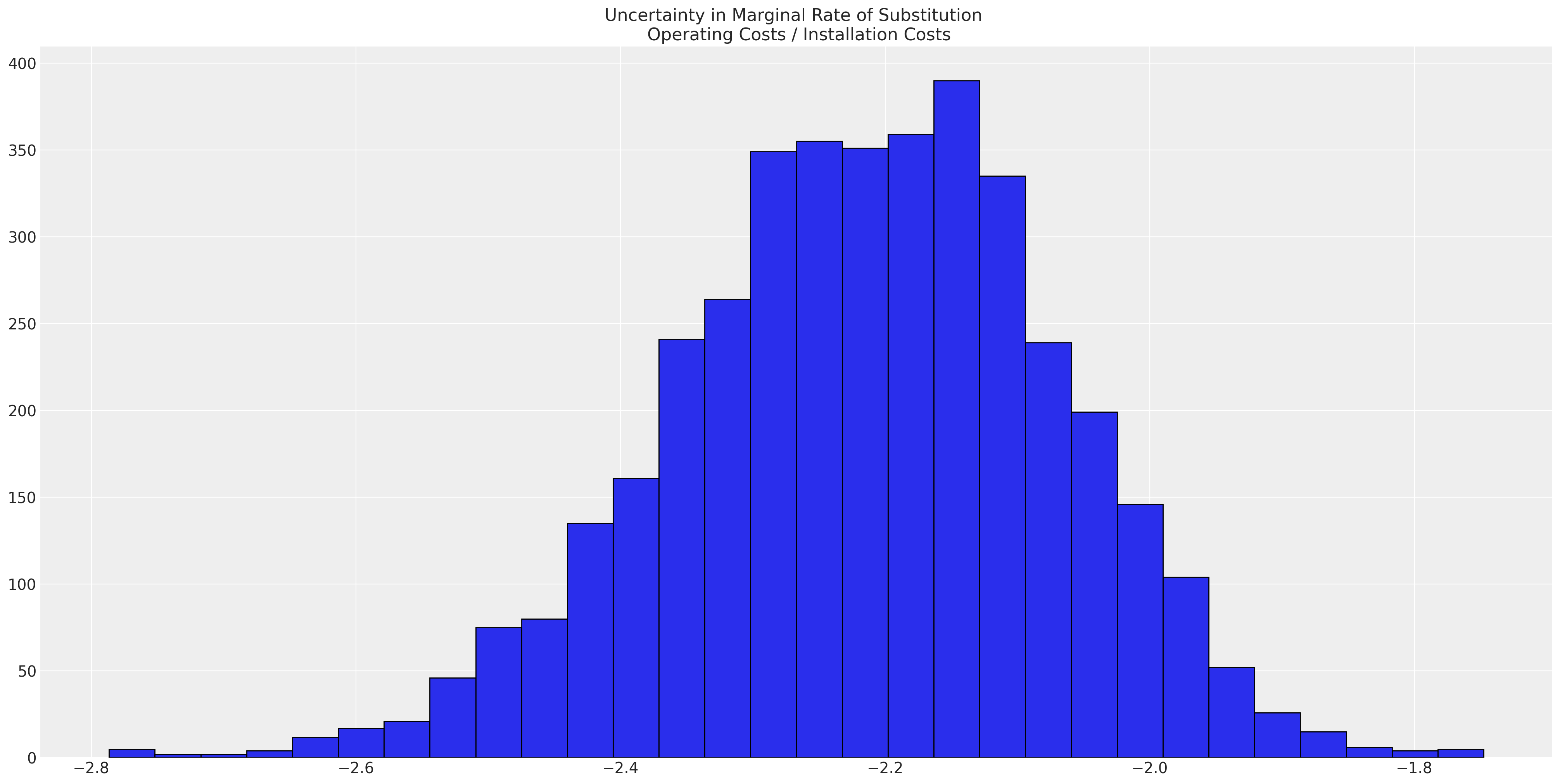
这表明,与一次性安装成本相比,持续运营成本每减少一个单位的价值几乎是其两倍。无论这是否有丝毫合理性,几乎都无关紧要,因为模型甚至没有接近捕捉到数据生成过程。但值得重复的是,效用的原生尺度并不是直接有意义的,但效用方程中系数的比率可以直接解释。
为了评估整体模型的充分性,我们可以依赖后验预测检查,以查看模型是否能够恢复对数据生成过程的近似。
idata_m1["posterior"]["p"].mean(dim=["chain", "draw", "obs"])
<xarray.DataArray 'p' (alts_probs: 5)>
array([0.08414602, 0.13748865, 0.26918857, 0.38213088, 0.12704589])
Coordinates:
  * alts_probs  (alts_probs) <U2 'ec' 'er' 'gc' 'gr' 'hp'
fig, axs = plt.subplots(1, 2, figsize=(20, 10))
ax = axs[0]
counts = wide_heating_df.groupby("depvar")["idcase"].count()
predicted_shares = idata_m1["posterior"]["p"].mean(dim=["chain", "draw", "obs"])
ci_lb = idata_m1["posterior"]["p"].quantile(0.025, dim=["chain", "draw", "obs"])
ci_ub = idata_m1["posterior"]["p"].quantile(0.975, dim=["chain", "draw", "obs"])
ax.scatter(ci_lb, ["ec", "er", "gc", "gr", "hp"], color="k", s=2)
ax.scatter(ci_ub, ["ec", "er", "gc", "gr", "hp"], color="k", s=2)
ax.scatter(
    counts / counts.sum(),
    ["ec", "er", "gc", "gr", "hp"],
    label="Observed Shares",
    color="red",
    s=100,
)
ax.hlines(
    ["ec", "er", "gc", "gr", "hp"], ci_lb, ci_ub, label="Predicted 95% Interval", color="black"
)
ax.legend()
ax.set_title("Observed V Predicted Shares")
az.plot_ppc(idata_m1, ax=axs[1])
axs[1].set_title("Posterior Predictive Checks")
ax.set_xlabel("Shares")
ax.set_ylabel("Heating System");
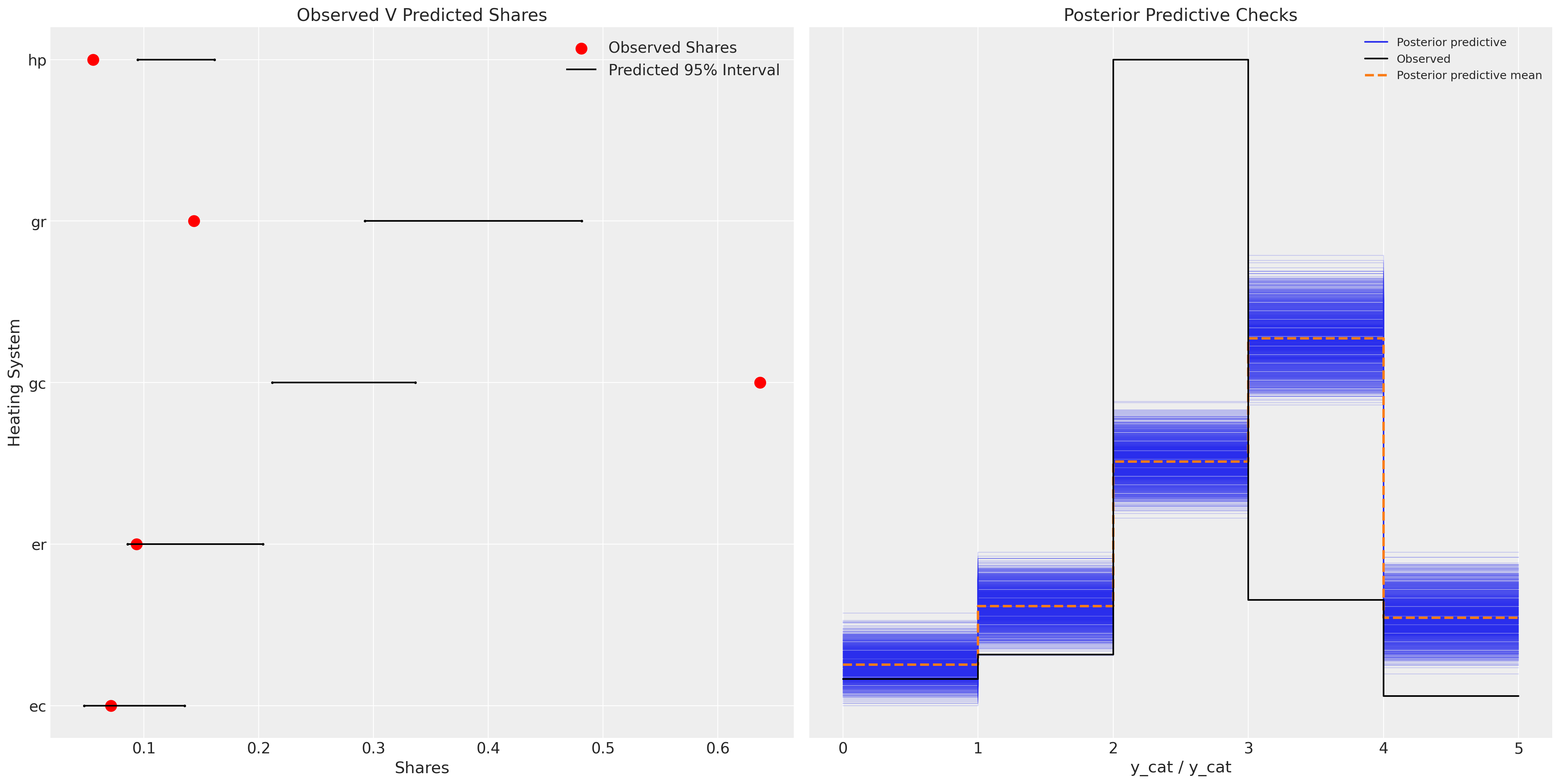
我们可以看到,这里的模型相当不足,并且未能很好地重现后验预测分布。
改进模型:添加替代特定截距#
我们可以通过为每个独特的选择添加截距项来解决先前模型规范中的一些问题,这些选择包括gr, gc, ec, er。这些项将通过允许我们控制产品之间效用度量的某些异质性来吸收上一个模型中看到的一些误差。
N = wide_heating_df.shape[0]
observed = pd.Categorical(wide_heating_df["depvar"]).codes

coords = {
    "alts_intercepts": ["ec", "er", "gc", "gr"],
    "alts_probs": ["ec", "er", "gc", "gr", "hp"],
    "obs": range(N),
}
with pm.Model(coords=coords) as model_2:
    beta_ic = pm.Normal("beta_ic", 0, 1)
    beta_oc = pm.Normal("beta_oc", 0, 1)
    alphas = pm.Normal("alpha", 0, 1, dims="alts_intercepts")

    ## Construct Utility matrix and Pivot using an intercept per alternative
    u0 = alphas[0] + beta_ic * wide_heating_df["ic.ec"] + beta_oc * wide_heating_df["oc.ec"]
    u1 = alphas[1] + beta_ic * wide_heating_df["ic.er"] + beta_oc * wide_heating_df["oc.er"]
    u2 = alphas[2] + beta_ic * wide_heating_df["ic.gc"] + beta_oc * wide_heating_df["oc.gc"]
    u3 = alphas[3] + beta_ic * wide_heating_df["ic.gr"] + beta_oc * wide_heating_df["oc.gr"]
    u4 = np.zeros(N)  # Outside Good
    s = pm.math.stack([u0, u1, u2, u3, u4]).T

    ## Apply Softmax Transform
    p_ = pm.Deterministic("p", pm.math.softmax(s, axis=1), dims=("obs", "alts_probs"))

    ## Likelihood
    choice_obs = pm.Categorical("y_cat", p=p_, observed=observed, dims="obs")

    idata_m2 = pm.sample_prior_predictive()
    idata_m2.extend(
        pm.sample(nuts_sampler="numpyro", idata_kwargs={"log_likelihood": True}, random_seed=103)
    )
    idata_m2.extend(pm.sample_posterior_predictive(idata_m2))


pm.model_to_graphviz(model_2)
Sampling: [alpha, beta_ic, beta_oc, y_cat]
/Users/nathanielforde/mambaforge/envs/pymc_examples_new/lib/python3.9/site-packages/pymc/sampling/mcmc.py:243: UserWarning: Use of external NUTS sampler is still experimental
  warnings.warn("Use of external NUTS sampler is still experimental", UserWarning)
Compiling...
Compilation time =  0:00:01.339706
Sampling...
Sampling time =  0:00:15.309789
Transforming variables...
Transformation time =  0:00:00.289041
Computing Log Likelihood...

az.summary(idata_m2, var_names=["beta_ic", "beta_oc", "alpha"])
| mean | sd | hdi_3% | hdi_97% | mcse_mean | mcse_sd | ess_bulk | ess_tail | r_hat | |
|---|---|---|---|---|---|---|---|---|---|
| beta_ic | 0.001 | 0.000 | -0.000 | 0.001 | 0.000 | 0.000 | 1215.0 | 1612.0 | 1.00 |
| beta_oc | -0.003 | 0.001 | -0.005 | -0.001 | 0.000 | 0.000 | 1379.0 | 1743.0 | 1.00 |
| alpha[ec] | 1.039 | 0.497 | 0.076 | 1.936 | 0.016 | 0.012 | 908.0 | 1054.0 | 1.00 |
| alpha[er] | 1.077 | 0.474 | 0.216 | 1.988 | 0.016 | 0.012 | 839.0 | 991.0 | 1.00 |
| alpha[gc] | 2.376 | 0.309 | 1.789 | 2.953 | 0.011 | 0.008 | 814.0 | 836.0 | 1.01 |
| alpha[gr] | 0.733 | 0.373 | -0.031 | 1.374 | 0.013 | 0.009 | 854.0 | 947.0 | 1.01 |
我们现在可以看到,这个模型在捕捉数据生成过程的各个方面表现得更好。
fig, axs = plt.subplots(1, 2, figsize=(20, 10))
ax = axs[0]
counts = wide_heating_df.groupby("depvar")["idcase"].count()
predicted_shares = idata_m2["posterior"]["p"].mean(dim=["chain", "draw", "obs"])
ci_lb = idata_m2["posterior"]["p"].quantile(0.025, dim=["chain", "draw", "obs"])
ci_ub = idata_m2["posterior"]["p"].quantile(0.975, dim=["chain", "draw", "obs"])

ax.scatter(ci_lb, ["ec", "er", "gc", "gr", "hp"], color="k", s=2)
ax.scatter(ci_ub, ["ec", "er", "gc", "gr", "hp"], color="k", s=2)
ax.scatter(
    counts / counts.sum(),
    ["ec", "er", "gc", "gr", "hp"],
    label="Observed Shares",
    color="red",
    s=100,
)
ax.hlines(
    ["ec", "er", "gc", "gr", "hp"], ci_lb, ci_ub, label="Predicted 95% Interval", color="black"
)
ax.legend()
ax.set_title("Observed V Predicted Shares")
az.plot_ppc(idata_m2, ax=axs[1])
axs[1].set_title("Posterior Predictive Checks")
ax.set_xlabel("Shares")
ax.set_ylabel("Heating System");
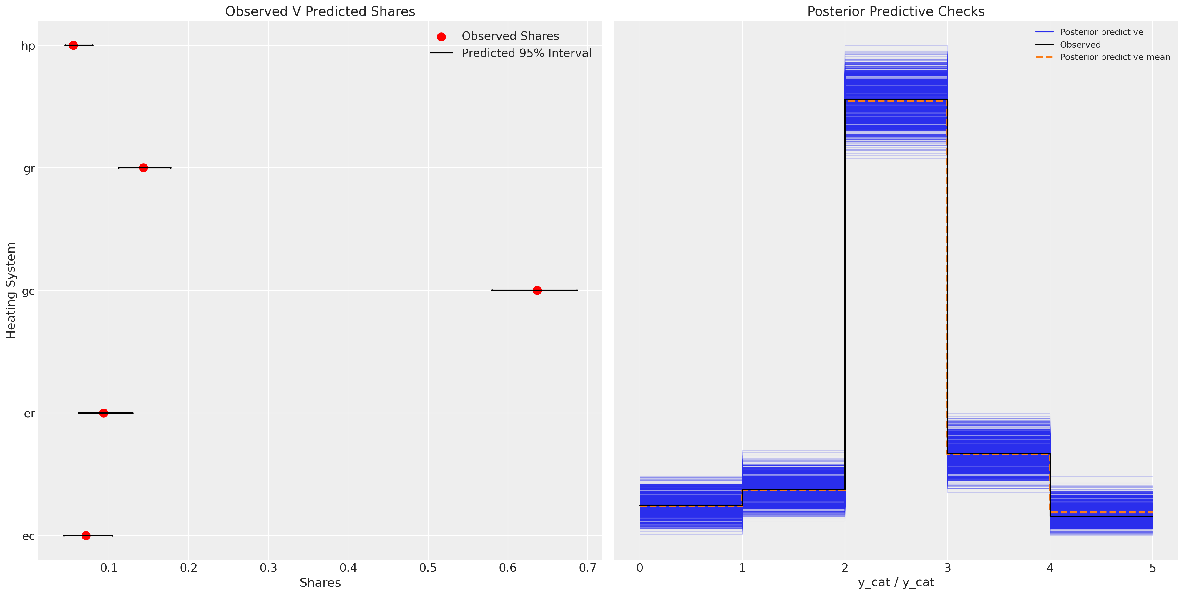
该模型代表了显著的改进。
实验模型:添加相关性结构#
我们可能会认为,替代商品之间存在相关性,我们也应该捕捉到这一点。我们可以通过在截距(或替代的beta参数)上放置一个多元正态先验来捕捉这些效应,只要它们存在。此外,我们还增加了关于收入效应如何影响每个替代品的效用的信息。
coords = {
    "alts_intercepts": ["ec", "er", "gc", "gr"],
    "alts_probs": ["ec", "er", "gc", "gr", "hp"],
    "obs": range(N),
}
with pm.Model(coords=coords) as model_3:
    ## Add data to experiment with changes later.
    ic_ec = pm.MutableData("ic_ec", wide_heating_df["ic.ec"])
    oc_ec = pm.MutableData("oc_ec", wide_heating_df["oc.ec"])
    ic_er = pm.MutableData("ic_er", wide_heating_df["ic.er"])
    oc_er = pm.MutableData("oc_er", wide_heating_df["oc.er"])

    beta_ic = pm.Normal("beta_ic", 0, 1)
    beta_oc = pm.Normal("beta_oc", 0, 1)
    beta_income = pm.Normal("beta_income", 0, 1, dims="alts_intercepts")
    chol, corr, stds = pm.LKJCholeskyCov(
        "chol", n=4, eta=2.0, sd_dist=pm.Exponential.dist(1.0, shape=4)
    )
    alphas = pm.MvNormal("alpha", mu=0, chol=chol, dims="alts_intercepts")

    u0 = alphas[0] + beta_ic * ic_ec + beta_oc * oc_ec + beta_income[0] * wide_heating_df["income"]
    u1 = alphas[1] + beta_ic * ic_er + beta_oc * oc_er + beta_income[1] * wide_heating_df["income"]
    u2 = (
        alphas[2]
        + beta_ic * wide_heating_df["ic.gc"]
        + beta_oc * wide_heating_df["oc.gc"]
        + beta_income[2] * wide_heating_df["income"]
    )
    u3 = (
        alphas[3]
        + beta_ic * wide_heating_df["ic.gr"]
        + beta_oc * wide_heating_df["oc.gr"]
        + beta_income[3] * wide_heating_df["income"]
    )
    u4 = np.zeros(N)  # pivot
    s = pm.math.stack([u0, u1, u2, u3, u4]).T

    p_ = pm.Deterministic("p", pm.math.softmax(s, axis=1), dims=("obs", "alts_probs"))
    choice_obs = pm.Categorical("y_cat", p=p_, observed=observed, dims="obs")

    idata_m3 = pm.sample_prior_predictive()
    idata_m3.extend(
        pm.sample(nuts_sampler="numpyro", idata_kwargs={"log_likelihood": True}, random_seed=100)
    )
    idata_m3.extend(pm.sample_posterior_predictive(idata_m3))


pm.model_to_graphviz(model_3)
Sampling: [alpha, beta_ic, beta_income, beta_oc, chol, y_cat]
/Users/nathanielforde/mambaforge/envs/pymc_examples_new/lib/python3.9/site-packages/pymc/sampling/mcmc.py:243: UserWarning: Use of external NUTS sampler is still experimental
  warnings.warn("Use of external NUTS sampler is still experimental", UserWarning)
Compiling...
Compilation time =  0:00:04.533953
Sampling...
Sampling time =  0:00:30.042792
Transforming variables...
Transformation time =  0:00:00.594139
Computing Log Likelihood...

绘制模型拟合图,我们看到了类似的情况。模型的预测性能并没有显著提高,而且我们增加了模型的复杂性。这种额外的复杂性应在模型评估指标(如AIC和WAIC)中受到惩罚。但通常情况下,产品之间的相关性是一些感兴趣的特征,与历史预测问题无关。
fig, axs = plt.subplots(1, 2, figsize=(20, 10))
ax = axs[0]
counts = wide_heating_df.groupby("depvar")["idcase"].count()
predicted_shares = idata_m3["posterior"]["p"].mean(dim=["chain", "draw", "obs"])
ci_lb = idata_m3["posterior"]["p"].quantile(0.025, dim=["chain", "draw", "obs"])
ci_ub = idata_m3["posterior"]["p"].quantile(0.975, dim=["chain", "draw", "obs"])

ax.scatter(ci_lb, ["ec", "er", "gc", "gr", "hp"], color="k", s=2)
ax.scatter(ci_ub, ["ec", "er", "gc", "gr", "hp"], color="k", s=2)
ax.scatter(
    counts / counts.sum(),
    ["ec", "er", "gc", "gr", "hp"],
    label="Observed Shares",
    color="red",
    s=100,
)
ax.hlines(
    ["ec", "er", "gc", "gr", "hp"], ci_lb, ci_ub, label="Predicted 95% Interval", color="black"
)
ax.legend()
ax.set_title("Observed V Predicted Shares")
az.plot_ppc(idata_m3, ax=axs[1])
axs[1].set_title("Posterior Predictive Checks")
ax.set_xlabel("Shares")
ax.set_ylabel("Heating System");
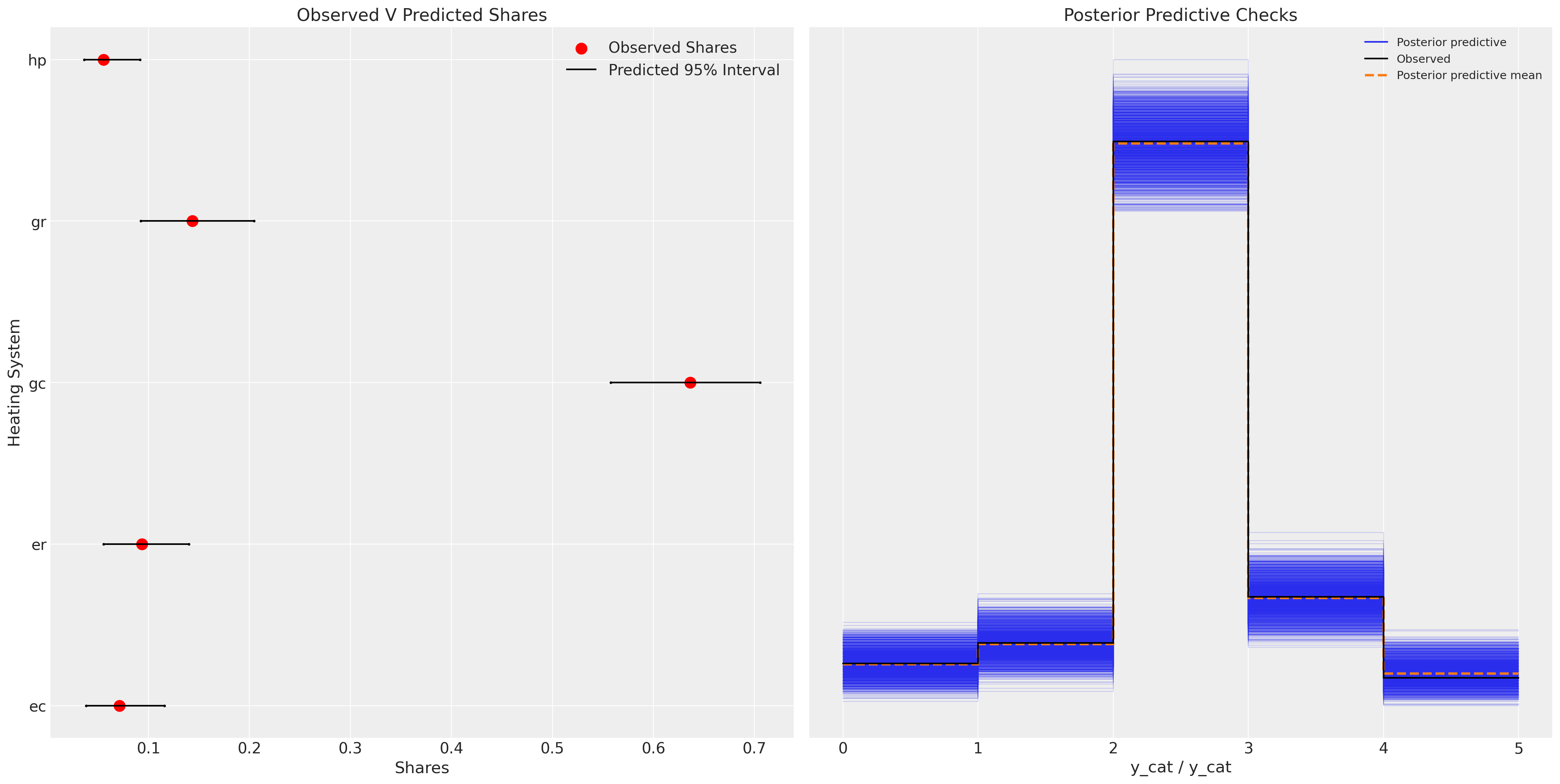
这种额外的复杂性可以提供信息,替代产品之间的关系程度将影响政策变化下的替代模式。此外,请注意在此模型规范下,参数beta_ic的期望值为0。这可能暗示了对安装成本现实的妥协,这种妥协在购买决策后不会以任何方式改变效用度量。
az.summary(
    idata_m3, var_names=["beta_income", "beta_ic", "beta_oc", "alpha", "chol_corr"], round_to=4
)
/Users/nathanielforde/mambaforge/envs/pymc_examples_new/lib/python3.9/site-packages/arviz/stats/diagnostics.py:592: RuntimeWarning: invalid value encountered in double_scalars
  (between_chain_variance / within_chain_variance + num_samples - 1) / (num_samples)
| mean | sd | hdi_3% | hdi_97% | mcse_mean | mcse_sd | ess_bulk | ess_tail | r_hat | |
|---|---|---|---|---|---|---|---|---|---|
| beta_income[ec] | 0.0971 | 0.1074 | -0.1025 | 0.3046 | 0.0035 | 0.0025 | 936.3265 | 1900.0530 | 1.0033 |
| beta_income[er] | 0.0655 | 0.1047 | -0.1187 | 0.2695 | 0.0036 | 0.0025 | 839.1058 | 1613.9147 | 1.0017 |
| beta_income[gc] | 0.0673 | 0.0867 | -0.1058 | 0.2202 | 0.0032 | 0.0023 | 722.9224 | 1321.0255 | 1.0028 |
| beta_income[gr] | -0.0318 | 0.0977 | -0.2220 | 0.1441 | 0.0034 | 0.0024 | 807.8161 | 1624.6096 | 1.0020 |
| beta_ic | 0.0004 | 0.0007 | -0.0009 | 0.0016 | 0.0000 | 0.0000 | 752.9909 | 914.0799 | 1.0019 |
| beta_oc | -0.0035 | 0.0015 | -0.0064 | -0.0007 | 0.0000 | 0.0000 | 1436.0405 | 2066.3187 | 1.0015 |
| alpha[ec] | 1.0354 | 1.0479 | -0.4211 | 3.0541 | 0.0470 | 0.0333 | 520.2449 | 1178.1694 | 1.0063 |
| alpha[er] | 1.2391 | 1.0751 | -0.3175 | 3.2426 | 0.0507 | 0.0358 | 441.6820 | 991.4928 | 1.0064 |
| alpha[gc] | 2.3718 | 0.7613 | 1.1220 | 3.7710 | 0.0366 | 0.0259 | 414.8905 | 699.3486 | 1.0073 |
| alpha[gr] | 1.2014 | 0.8524 | -0.0952 | 2.8006 | 0.0402 | 0.0284 | 442.3913 | 1198.3044 | 1.0053 |
| chol_corr[0, 0] | 1.0000 | 0.0000 | 1.0000 | 1.0000 | 0.0000 | 0.0000 | 4000.0000 | 4000.0000 | NaN |
| chol_corr[0, 1] | 0.1184 | 0.3671 | -0.5402 | 0.7923 | 0.0074 | 0.0062 | 2518.0052 | 2043.9328 | 1.0015 |
| chol_corr[0, 2] | 0.1427 | 0.3705 | -0.5480 | 0.7769 | 0.0093 | 0.0066 | 1673.7845 | 1975.7307 | 1.0020 |
| chol_corr[0, 3] | 0.1157 | 0.3753 | -0.5676 | 0.7683 | 0.0079 | 0.0056 | 2319.4753 | 2119.7780 | 1.0012 |
| chol_corr[1, 0] | 0.1184 | 0.3671 | -0.5402 | 0.7923 | 0.0074 | 0.0062 | 2518.0052 | 2043.9328 | 1.0015 |
| chol_corr[1, 1] | 1.0000 | 0.0000 | 1.0000 | 1.0000 | 0.0000 | 0.0000 | 4239.6296 | 4000.0000 | 0.9996 |
| chol_corr[1, 2] | 0.1675 | 0.3483 | -0.4430 | 0.8095 | 0.0079 | 0.0056 | 1978.9399 | 1538.2851 | 1.0011 |
| chol_corr[1, 3] | 0.1526 | 0.3561 | -0.4722 | 0.7963 | 0.0070 | 0.0050 | 2595.1991 | 3126.5524 | 1.0014 |
| chol_corr[2, 0] | 0.1427 | 0.3705 | -0.5480 | 0.7769 | 0.0093 | 0.0066 | 1673.7845 | 1975.7307 | 1.0020 |
| chol_corr[2, 1] | 0.1675 | 0.3483 | -0.4430 | 0.8095 | 0.0079 | 0.0056 | 1978.9399 | 1538.2851 | 1.0011 |
| chol_corr[2, 2] | 1.0000 | 0.0000 | 1.0000 | 1.0000 | 0.0000 | 0.0000 | 3929.0431 | 4000.0000 | 1.0007 |
| chol_corr[2, 3] | 0.1757 | 0.3411 | -0.4384 | 0.7867 | 0.0071 | 0.0051 | 2260.6724 | 2564.2728 | 1.0017 |
| chol_corr[3, 0] | 0.1157 | 0.3753 | -0.5676 | 0.7683 | 0.0079 | 0.0056 | 2319.4753 | 2119.7780 | 1.0012 |
| chol_corr[3, 1] | 0.1526 | 0.3561 | -0.4722 | 0.7963 | 0.0070 | 0.0050 | 2595.1991 | 3126.5524 | 1.0014 |
| chol_corr[3, 2] | 0.1757 | 0.3411 | -0.4384 | 0.7867 | 0.0071 | 0.0051 | 2260.6724 | 2564.2728 | 1.0017 |
| chol_corr[3, 3] | 1.0000 | 0.0000 | 1.0000 | 1.0000 | 0.0000 | 0.0000 | 3954.4789 | 3702.0363 | 1.0001 |
在这个模型中,我们看到边际替代率表明,运营成本每增加一美元对效用计算的影响几乎是安装成本类似增加的17倍。这在某种程度上是有道理的,因为我们预期安装成本是一次性费用,我们对此已经相当接受。
post = az.extract(idata_m3)
substitution_rate = post["beta_oc"] / post["beta_ic"]
substitution_rate.mean().item()
17.581376035151784
市场干预与市场份额预测#
我们还可以使用这些类型的模型来预测在改变价格策略时的市场份额。
with model_3:
    # update values of predictors with new 20% price increase in operating costs for electrical options
    pm.set_data({"oc_ec": wide_heating_df["oc.ec"] * 1.2, "oc_er": wide_heating_df["oc.er"] * 1.2})
    # use the updated values and predict outcomes and probabilities:
    idata_new_policy = pm.sample_posterior_predictive(
        idata_m3,
        var_names=["p", "y_cat"],
        return_inferencedata=True,
        predictions=True,
        extend_inferencedata=False,
        random_seed=100,
    )

idata_new_policy
-
<xarray.Dataset> Dimensions: (chain: 4, draw: 1000, obs: 900, alts_probs: 5) Coordinates: * chain (chain) int64 0 1 2 3 * draw (draw) int64 0 1 2 3 4 5 6 7 ... 992 993 994 995 996 997 998 999 * obs (obs) int64 0 1 2 3 4 5 6 7 ... 892 893 894 895 896 897 898 899 * alts_probs (alts_probs) <U2 'ec' 'er' 'gc' 'gr' 'hp' Data variables: p (chain, draw, obs, alts_probs) float64 0.04832 ... 0.05605 y_cat (chain, draw, obs) int64 2 4 4 2 1 2 2 2 2 ... 2 3 3 3 2 1 2 4 2 Attributes: created_at: 2023-07-13T17:30:54.332027 arviz_version: 0.15.1 inference_library: pymc inference_library_version: 5.3.0 -
<xarray.Dataset>
Dimensions:      (ic_ec_dim_0: 900, oc_ec_dim_0: 900, ic_er_dim_0: 900,
                  oc_er_dim_0: 900)
Coordinates:
  * ic_ec_dim_0  (ic_ec_dim_0) int64 0 1 2 3 4 5 6 ... 894 895 896 897 898 899
  * oc_ec_dim_0  (oc_ec_dim_0) int64 0 1 2 3 4 5 6 ... 894 895 896 897 898 899
  * ic_er_dim_0  (ic_er_dim_0) int64 0 1 2 3 4 5 6 ... 894 895 896 897 898 899
  * oc_er_dim_0  (oc_er_dim_0) int64 0 1 2 3 4 5 6 ... 894 895 896 897 898 899
Data variables:
    ic_ec        (ic_ec_dim_0) float64 859.9 796.8 719.9 ... 842.8 799.8 967.9
    oc_ec        (oc_ec_dim_0) float64 664.0 624.3 526.9 ... 574.6 594.2 622.4
    ic_er        (ic_er_dim_0) float64 995.8 894.7 900.1 ... 1.123e+03 1.092e+03
    oc_er        (oc_er_dim_0) float64 606.7 583.8 485.7 ... 538.3 481.9 550.2
Attributes:
    created_at:                 2023-07-13T17:30:54.333501
    arviz_version:              0.15.1
    inference_library:          pymc
    inference_library_version:  5.3.0
idata_new_policy["predictions"]["p"].mean(dim=["chain", "draw", "obs"])
<xarray.DataArray 'p' (alts_probs: 5)>
array([0.05383866, 0.07239016, 0.66253495, 0.1482966 , 0.06293963])
Coordinates:
  * alts_probs  (alts_probs) <U2 'ec' 'er' 'gc' 'gr' 'hp'
fig, ax = plt.subplots(1, figsize=(20, 10))
counts = wide_heating_df.groupby("depvar")["idcase"].count()
new_predictions = idata_new_policy["predictions"]["p"].mean(dim=["chain", "draw", "obs"]).values
ci_lb = idata_m3["posterior"]["p"].quantile(0.025, dim=["chain", "draw", "obs"])
ci_ub = idata_m3["posterior"]["p"].quantile(0.975, dim=["chain", "draw", "obs"])
ax.scatter(ci_lb, ["ec", "er", "gc", "gr", "hp"], color="k", s=2)
ax.scatter(ci_ub, ["ec", "er", "gc", "gr", "hp"], color="k", s=2)
ax.scatter(
    new_predictions,
    ["ec", "er", "gc", "gr", "hp"],
    color="green",
    label="New Policy Predicted Share",
    s=100,
)
ax.scatter(
    counts / counts.sum(),
    ["ec", "er", "gc", "gr", "hp"],
    label="Observed Shares",
    color="red",
    s=100,
)
ax.hlines(
    ["ec", "er", "gc", "gr", "hp"],
    ci_lb,
    ci_ub,
    label="Predicted 95% Credible Interval Old Policy",
    color="black",
)
ax.set_title("Predicted Market Shares under Old and New Pricing Policy", fontsize=20)
ax.set_xlabel("Market Share")
ax.legend();
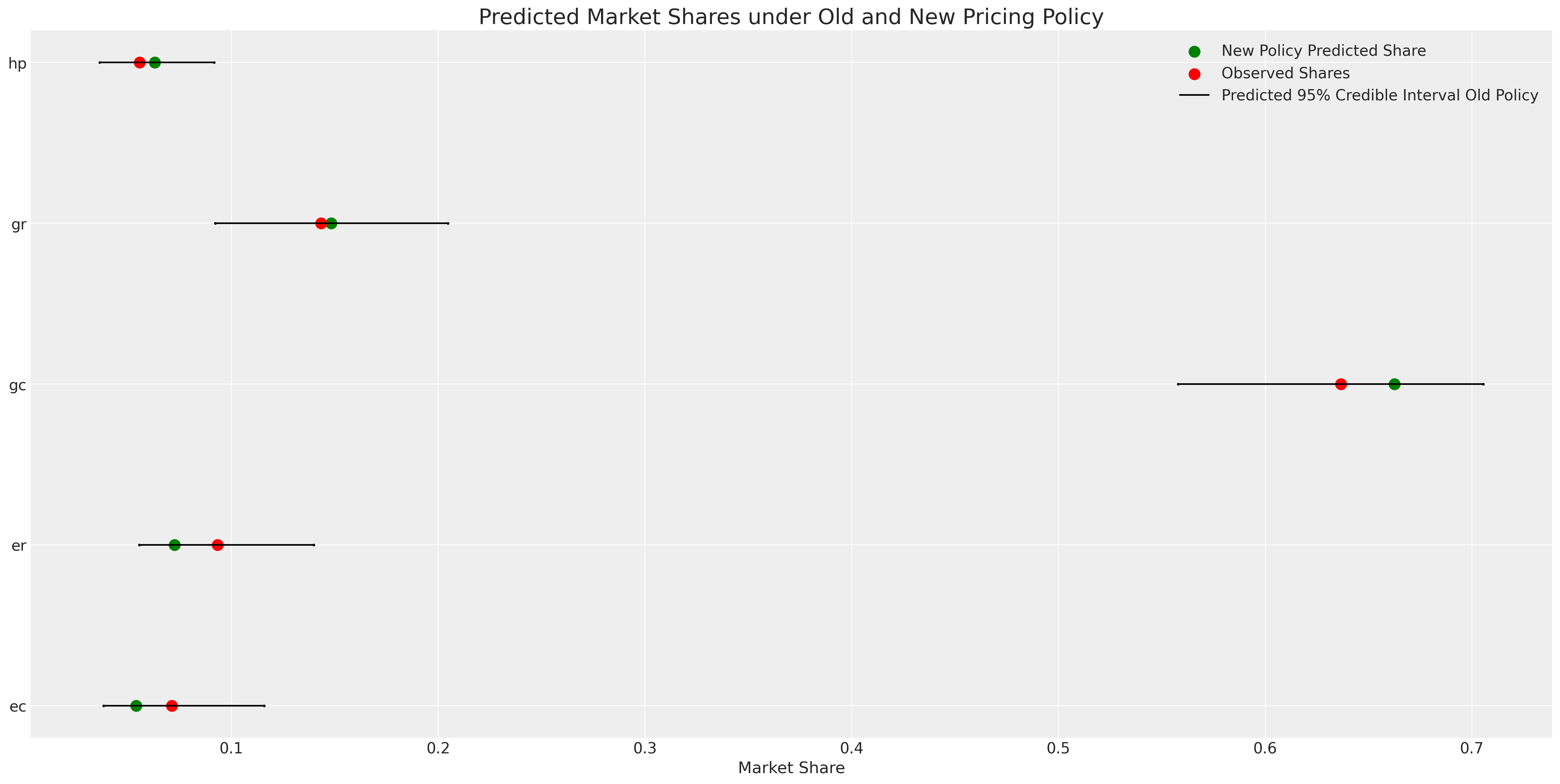
在这里,我们可以如预期地看到,电力选项的运营成本上升对它们的预测市场份额产生了负面影响。
比较模型#
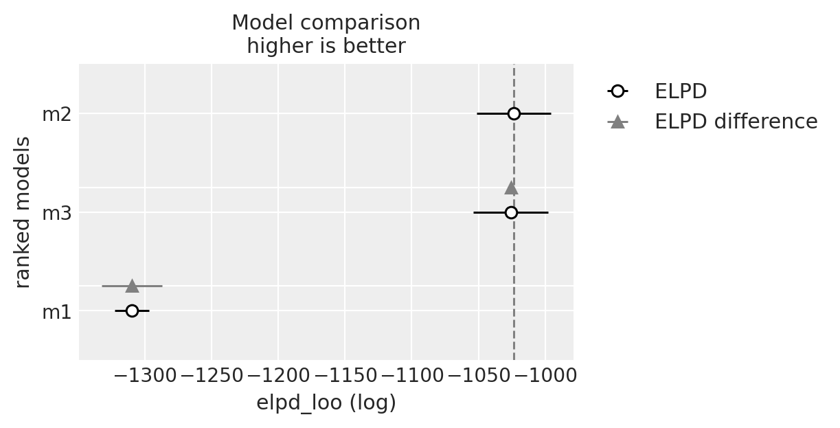
我们现在将评估所有三个模型的预测性能。在原始数据上的预测性能是一个很好的基准,表明模型已经适当地捕捉了数据生成过程。但正如我们所见,这并不是这些模型中唯一值得关注的特征。这些模型对我们的理论信念、决策过程的观点以及选择场景的元素非常敏感。
compare = az.compare({"m1": idata_m1, "m2": idata_m2, "m3": idata_m3})
compare
| rank | elpd_loo | p_loo | elpd_diff | weight | se | dse | warning | scale | |
|---|---|---|---|---|---|---|---|---|---|
| m2 | 0 | -1023.600927 | 4.964862 | 0.000000 | 1.000000e+00 | 27.802379 | 0.000000 | False | log |
| m3 | 1 | -1025.830780 | 9.954792 | 2.229854 | 2.220446e-16 | 28.086804 | 2.070976 | False | log |
| m1 | 2 | -1309.610895 | 1.196878 | 286.009968 | 0.000000e+00 | 12.933024 | 22.677606 | False | log |
az.plot_compare(compare)
<Axes: title={'center': 'Model comparison\nhigher is better'}, xlabel='elpd_loo (log)', ylabel='ranked models'>
选择饼干而非重复选择:混合Logit模型#
转移到另一个例子,我们看到一个选择场景,其中同一个人在不同替代品中反复被调查他们对饼干的选择。这使我们有机会通过为每个产品添加个人系数来评估个人的偏好。
try:
    c_df = pd.read_csv("../data/cracker_choice_short.csv")
except:
    c_df = pd.read_csv(pm.get_data("cracker_choice_short.csv"))
columns = [c for c in c_df.columns if c != "Unnamed: 0"]
c_df[columns]
| personId | disp.sunshine | disp.keebler | disp.nabisco | disp.private | feat.sunshine | feat.keebler | feat.nabisco | feat.private | price.sunshine | price.keebler | price.nabisco | price.private | choice | lastChoice | personChoiceId | choiceId | |
|---|---|---|---|---|---|---|---|---|---|---|---|---|---|---|---|---|---|
| 0 | 1 | 0 | 0 | 0 | 0 | 0 | 0 | 0 | 0 | 0.99 | 1.09 | 0.99 | 0.71 | nabisco | nabisco | 1 | 1 |
| 1 | 1 | 1 | 0 | 0 | 0 | 0 | 0 | 0 | 0 | 0.49 | 1.09 | 1.09 | 0.78 | sunshine | nabisco | 2 | 2 |
| 2 | 1 | 0 | 0 | 0 | 0 | 0 | 0 | 0 | 0 | 1.03 | 1.09 | 0.89 | 0.78 | nabisco | sunshine | 3 | 3 |
| 3 | 1 | 0 | 0 | 0 | 0 | 0 | 0 | 0 | 0 | 1.09 | 1.09 | 1.19 | 0.64 | nabisco | nabisco | 4 | 4 |
| 4 | 1 | 0 | 0 | 0 | 0 | 0 | 0 | 0 | 0 | 0.89 | 1.09 | 1.19 | 0.84 | nabisco | nabisco | 5 | 5 |
| ... | ... | ... | ... | ... | ... | ... | ... | ... | ... | ... | ... | ... | ... | ... | ... | ... | ... |
| 3151 | 136 | 0 | 0 | 0 | 0 | 0 | 0 | 0 | 0 | 1.09 | 1.19 | 0.99 | 0.55 | private | private | 9 | 3152 |
| 3152 | 136 | 0 | 0 | 0 | 1 | 0 | 0 | 0 | 0 | 0.78 | 1.35 | 1.04 | 0.65 | private | private | 10 | 3153 |
| 3153 | 136 | 0 | 0 | 0 | 0 | 0 | 0 | 0 | 0 | 1.09 | 1.17 | 1.29 | 0.59 | private | private | 11 | 3154 |
| 3154 | 136 | 0 | 0 | 0 | 0 | 0 | 0 | 0 | 0 | 1.09 | 1.22 | 1.29 | 0.59 | private | private | 12 | 3155 |
| 3155 | 136 | 0 | 0 | 0 | 0 | 0 | 0 | 0 | 0 | 1.29 | 1.04 | 1.23 | 0.59 | private | private | 13 | 3156 |
3156 行 × 17 列
c_df.groupby("personId")[["choiceId"]].count().T
| personId | 1 | 2 | 3 | 4 | 5 | 6 | 7 | 8 | 9 | 10 | ... | 127 | 128 | 129 | 130 | 131 | 132 | 133 | 134 | 135 | 136 |
|---|---|---|---|---|---|---|---|---|---|---|---|---|---|---|---|---|---|---|---|---|---|
| choiceId | 15 | 15 | 13 | 28 | 13 | 27 | 16 | 25 | 18 | 40 | ... | 17 | 25 | 31 | 31 | 29 | 21 | 26 | 13 | 14 | 13 |
1 行 × 136 列
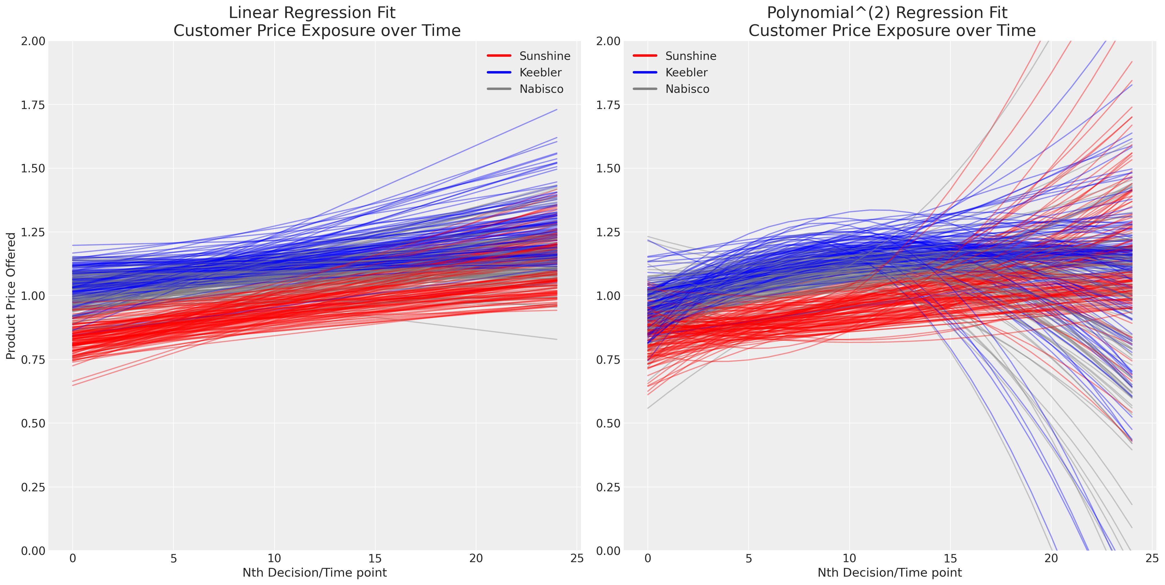
随着时间的推移,重复选择的出现使问题变得复杂。我们现在必须处理个人口味的问题以及在竞争环境中定价的演变或动态效应。绘制每个人对品牌价格连续接触的简单线性和多项式拟合图,似乎表明(a)定价区分了产品供应,以及(b)定价随时间演变。
fig, axs = plt.subplots(1, 2, figsize=(20, 10))
axs = axs.flatten()
map_color = {"nabisco": "red", "keebler": "blue", "sunshine": "purple", "private": "orange"}


for i in c_df["personId"].unique():
    temp = c_df[c_df["personId"] == i].copy(deep=True)
    temp["color"] = temp["choice"].map(map_color)
    predict = np.poly1d(np.polyfit(temp["personChoiceId"], temp["price.sunshine"], deg=1))
    axs[0].plot(predict(range(25)), color="red", label="Sunshine", alpha=0.4)
    predict = np.poly1d(np.polyfit(temp["personChoiceId"], temp["price.keebler"], deg=1))
    axs[0].plot(predict(range(25)), color="blue", label="Keebler", alpha=0.4)
    predict = np.poly1d(np.polyfit(temp["personChoiceId"], temp["price.nabisco"], deg=1))
    axs[0].plot(predict(range(25)), color="grey", label="Nabisco", alpha=0.4)

    predict = np.poly1d(np.polyfit(temp["personChoiceId"], temp["price.sunshine"], deg=2))
    axs[1].plot(predict(range(25)), color="red", label="Sunshine", alpha=0.4)
    predict = np.poly1d(np.polyfit(temp["personChoiceId"], temp["price.keebler"], deg=2))
    axs[1].plot(predict(range(25)), color="blue", label="Keebler", alpha=0.4)
    predict = np.poly1d(np.polyfit(temp["personChoiceId"], temp["price.nabisco"], deg=2))
    axs[1].plot(predict(range(25)), color="grey", label="Nabisco", alpha=0.4)

axs[0].set_title("Linear Regression Fit \n Customer Price Exposure over Time", fontsize=20)
axs[1].set_title("Polynomial^(2) Regression Fit \n Customer Price Exposure over Time", fontsize=20)
axs[0].set_xlabel("Nth Decision/Time point")
axs[1].set_xlabel("Nth Decision/Time point")
axs[0].set_ylabel("Product Price Offered")
axs[1].set_ylim(0, 2)
axs[0].set_ylim(0, 2)

colors = ["red", "blue", "grey"]
lines = [Line2D([0], [0], color=c, linewidth=3, linestyle="-") for c in colors]
labels = ["Sunshine", "Keebler", "Nabisco"]
axs[0].legend(lines, labels)
axs[1].legend(lines, labels);
我们现在将模拟个体口味如何进入离散选择问题,但忽略时间维度或系统中价格的内在复杂性。有一些基本离散选择模型的适应版本,旨在解决这些复杂性中的每一个。我们将时间动态作为建议的练习留给读者。
N = c_df.shape[0]
observed = pd.Categorical(c_df["choice"]).codes
person_indx, uniques = pd.factorize(c_df["personId"])

coords = {
    "alts_intercepts": ["sunshine", "keebler", "nabisco"],
    "alts_probs": ["sunshine", "keebler", "nabisco", "private"],
    "individuals": uniques,
    "obs": range(N),
}
with pm.Model(coords=coords) as model_4:
    beta_feat = pm.TruncatedNormal("beta_feat", 0, 1, upper=10, lower=0)
    beta_disp = pm.TruncatedNormal("beta_disp", 0, 1, upper=10, lower=0)
    ## Stronger Prior on Price to ensure an increase in price negatively impacts utility
    beta_price = pm.TruncatedNormal("beta_price", 0, 1, upper=0, lower=-10)
    alphas = pm.Normal("alpha", 0, 1, dims="alts_intercepts")
    beta_individual = pm.Normal("beta_individual", 0, 0.05, dims=("individuals", "alts_intercepts"))

    u0 = (
        (alphas[0] + beta_individual[person_indx, 0])
        + beta_disp * c_df["disp.sunshine"]
        + beta_feat * c_df["feat.sunshine"]
        + beta_price * c_df["price.sunshine"]
    )
    u1 = (
        (alphas[1] + beta_individual[person_indx, 1])
        + beta_disp * c_df["disp.keebler"]
        + beta_feat * c_df["feat.keebler"]
        + beta_price * c_df["price.keebler"]
    )
    u2 = (
        (alphas[2] + beta_individual[person_indx, 2])
        + beta_disp * c_df["disp.nabisco"]
        + beta_feat * c_df["feat.nabisco"]
        + beta_price * c_df["price.nabisco"]
    )
    u3 = np.zeros(N)  # Outside Good
    s = pm.math.stack([u0, u1, u2, u3]).T
    # Reconstruct the total data

    ## Apply Softmax Transform
    p_ = pm.Deterministic("p", pm.math.softmax(s, axis=1), dims=("obs", "alts_probs"))

    ## Likelihood
    choice_obs = pm.Categorical("y_cat", p=p_, observed=observed, dims="obs")

    idata_m4 = pm.sample_prior_predictive()
    idata_m4.extend(
        pm.sample(nuts_sampler="numpyro", idata_kwargs={"log_likelihood": True}, random_seed=103)
    )
    idata_m4.extend(pm.sample_posterior_predictive(idata_m4))


pm.model_to_graphviz(model_4)
Sampling: [alpha, beta_disp, beta_feat, beta_individual, beta_price, y_cat]
/Users/nathanielforde/mambaforge/envs/pymc_examples_new/lib/python3.9/site-packages/pymc/sampling/mcmc.py:243: UserWarning: Use of external NUTS sampler is still experimental
  warnings.warn("Use of external NUTS sampler is still experimental", UserWarning)
Compiling...
Compilation time =  0:00:02.628050
Sampling...
Sampling time =  0:00:11.040460
Transforming variables...
Transformation time =  0:00:01.419801
Computing Log Likelihood...

az.summary(idata_m4, var_names=["beta_disp", "beta_feat", "beta_price", "alpha", "beta_individual"])
| mean | sd | hdi_3% | hdi_97% | mcse_mean | mcse_sd | ess_bulk | ess_tail | r_hat | |
|---|---|---|---|---|---|---|---|---|---|
| beta_disp | 0.023 | 0.021 | 0.000 | 0.061 | 0.000 | 0.000 | 5386.0 | 2248.0 | 1.0 |
| beta_feat | 0.019 | 0.018 | 0.000 | 0.052 | 0.000 | 0.000 | 6417.0 | 2283.0 | 1.0 |
| beta_price | -0.021 | 0.020 | -0.059 | -0.000 | 0.000 | 0.000 | 4281.0 | 2277.0 | 1.0 |
| alpha[sunshine] | -0.054 | 0.096 | -0.243 | 0.119 | 0.002 | 0.001 | 3632.0 | 3220.0 | 1.0 |
| alpha[keebler] | 2.023 | 0.073 | 1.886 | 2.159 | 0.001 | 0.001 | 3302.0 | 2894.0 | 1.0 |
| ... | ... | ... | ... | ... | ... | ... | ... | ... | ... |
| beta_individual[135, keebler] | 0.012 | 0.048 | -0.077 | 0.104 | 0.000 | 0.001 | 10419.0 | 3135.0 | 1.0 |
| beta_individual[135, nabisco] | -0.009 | 0.051 | -0.108 | 0.081 | 0.000 | 0.001 | 10504.0 | 2555.0 | 1.0 |
| beta_individual[136, sunshine] | -0.002 | 0.049 | -0.089 | 0.096 | 0.001 | 0.001 | 7867.0 | 2729.0 | 1.0 |
| beta_individual[136, keebler] | -0.018 | 0.048 | -0.112 | 0.071 | 0.001 | 0.001 | 7684.0 | 2845.0 | 1.0 |
| beta_individual[136, nabisco] | 0.020 | 0.050 | -0.072 | 0.114 | 0.001 | 0.001 | 8252.0 | 2559.0 | 1.0 |
414 行 × 9 列
我们学到了什么?我们对价格系数施加了负斜率,但给了它一个广泛的先验。我们可以看到,数据足以大大缩小系数的可能范围。
az.plot_dist_comparison(idata_m4, var_names=["beta_price"]);
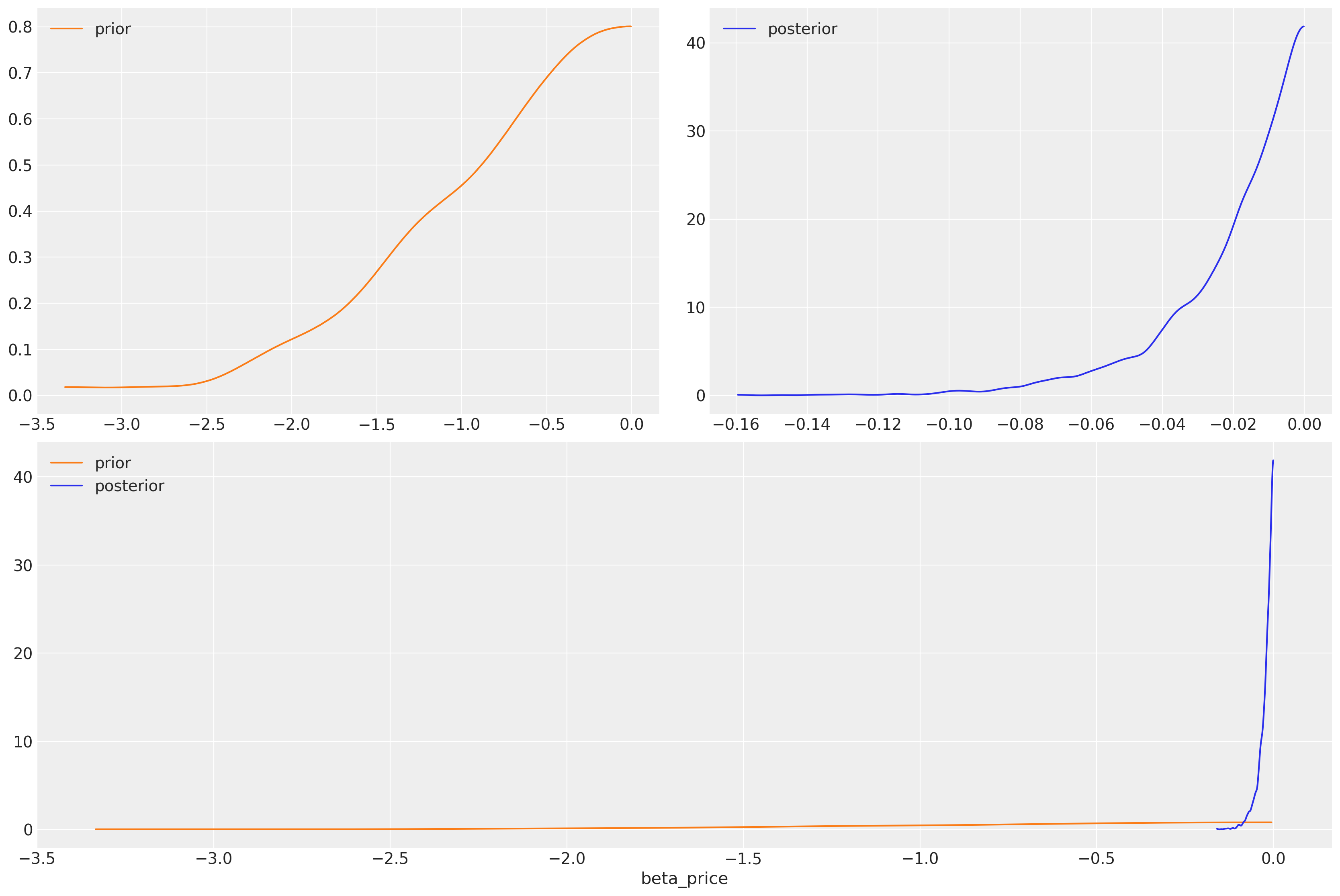
我们已经明确地设置了一个负面的价格先验,并恢复了一个更符合理性选择基本理论的参数规范。价格的影响应该对效用产生负面影响。这里的先验灵活性是关键,它有助于结合关于选择过程中涉及的理论知识。先验对于构建更好的决策过程图景非常重要,在这个设置中忽视它们的价值将是愚蠢的。
fig, axs = plt.subplots(1, 2, figsize=(20, 10))
ax = axs[0]
counts = c_df.groupby("choice")["choiceId"].count()
labels = c_df.groupby("choice")["choiceId"].count().index
predicted_shares = idata_m4["posterior"]["p"].mean(dim=["chain", "draw", "obs"])
ci_lb = idata_m4["posterior"]["p"].quantile(0.025, dim=["chain", "draw", "obs"])
ci_ub = idata_m4["posterior"]["p"].quantile(0.975, dim=["chain", "draw", "obs"])
ax.scatter(ci_lb, labels, color="k", s=2)
ax.scatter(ci_ub, labels, color="k", s=2)
ax.scatter(
    counts / counts.sum(),
    labels,
    label="Observed Shares",
    color="red",
    s=100,
)
ax.scatter(
    predicted_shares,
    labels,
    label="Predicted Mean",
    color="green",
    s=100,
)
ax.hlines(
    labels,
    ci_lb,
    ci_ub,
    label="Predicted 95% Interval",
    color="black",
)
ax.legend()
ax.set_title("Observed V Predicted Shares")
az.plot_ppc(idata_m4, ax=axs[1])
axs[1].set_title("Posterior Predictive Checks")
ax.set_xlabel("Shares")
ax.set_ylabel("Crackers");
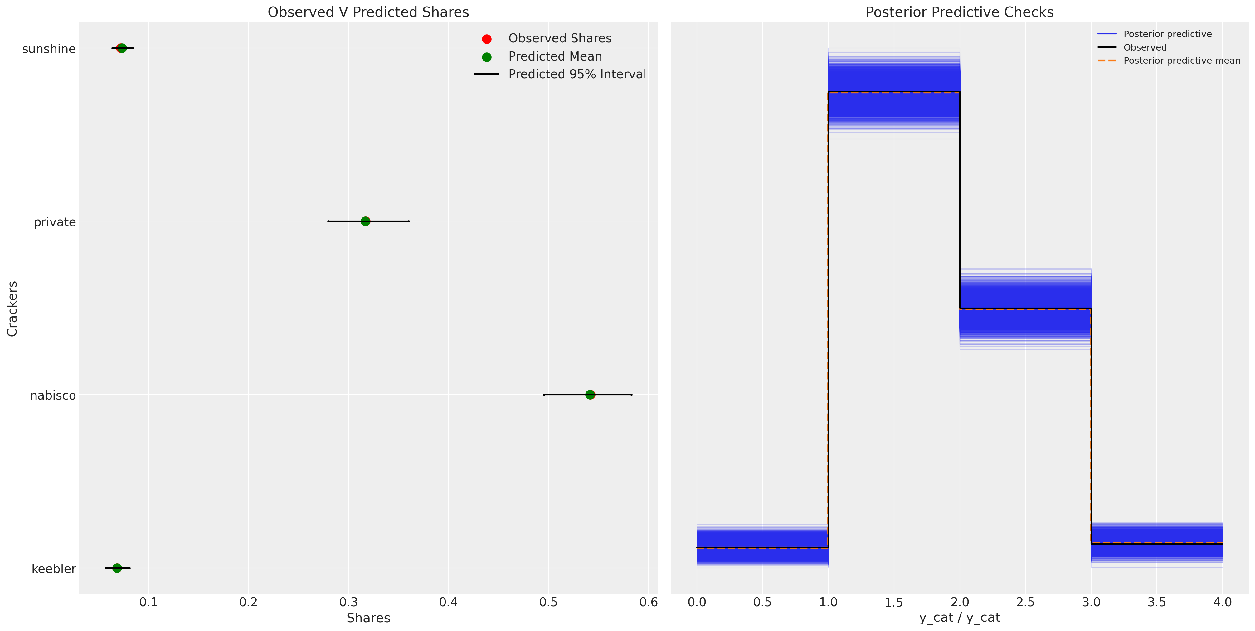
我们现在还可以恢复模型估计的个体之间在特定饼干选择上的差异。更准确地说,我们将绘制个体特定贡献如何影响饼干选择的偏好。
idata_m4
-
<xarray.Dataset> Dimensions: (chain: 4, draw: 1000, alts_intercepts: 3, individuals: 136, obs: 3156, alts_probs: 4) Coordinates: * chain (chain) int64 0 1 2 3 * draw (draw) int64 0 1 2 3 4 5 6 ... 993 994 995 996 997 998 999 * alts_intercepts (alts_intercepts) <U8 'sunshine' 'keebler' 'nabisco' * individuals (individuals) int64 1 2 3 4 5 6 ... 131 132 133 134 135 136 * obs (obs) int64 0 1 2 3 4 5 6 ... 3150 3151 3152 3153 3154 3155 * alts_probs (alts_probs) <U8 'sunshine' 'keebler' 'nabisco' 'private' Data variables: alpha (chain, draw, alts_intercepts) float64 -0.03604 ... 1.472 beta_individual (chain, draw, individuals, alts_intercepts) float64 -0.0... beta_feat (chain, draw) float64 0.008284 0.00381 ... 0.06727 0.0183 beta_disp (chain, draw) float64 0.02731 0.02334 ... 0.003561 0.001434 beta_price (chain, draw) float64 -0.01967 -0.08042 ... -0.01557 p (chain, draw, obs, alts_probs) float64 0.05909 ... 0.07105 Attributes: created_at: 2023-07-13T17:31:22.499390 arviz_version: 0.15.1 -
<xarray.Dataset> Dimensions: (chain: 4, draw: 1000, obs: 3156) Coordinates: * chain (chain) int64 0 1 2 3 * draw (draw) int64 0 1 2 3 4 5 6 7 8 ... 992 993 994 995 996 997 998 999 * obs (obs) int64 0 1 2 3 4 5 6 7 ... 3149 3150 3151 3152 3153 3154 3155 Data variables: y_cat (chain, draw, obs) int64 2 0 1 2 2 1 2 2 1 1 ... 2 1 2 2 1 1 2 2 1 Attributes: created_at: 2023-07-13T17:31:45.522950 arviz_version: 0.15.1 inference_library: pymc inference_library_version: 5.3.0 -
<xarray.Dataset> Dimensions: (chain: 4, draw: 1000, y_cat_dim_0: 1, y_cat_dim_1: 3156) Coordinates: * chain (chain) int64 0 1 2 3 * draw (draw) int64 0 1 2 3 4 5 6 7 ... 993 994 995 996 997 998 999 * y_cat_dim_0 (y_cat_dim_0) int64 0 * y_cat_dim_1 (y_cat_dim_1) int64 0 1 2 3 4 5 ... 3151 3152 3153 3154 3155 Data variables: y_cat (chain, draw, y_cat_dim_0, y_cat_dim_1) float64 -0.5664 ... ... Attributes: created_at: 2023-07-13T17:31:22.503457 arviz_version: 0.15.1 -
<xarray.Dataset> Dimensions: (chain: 4, draw: 1000) Coordinates: * chain (chain) int64 0 1 2 3 * draw (draw) int64 0 1 2 3 4 5 6 ... 993 994 995 996 997 998 999 Data variables: acceptance_rate (chain, draw) float64 0.7536 1.0 0.832 ... 0.5635 0.7482 step_size (chain, draw) float64 0.3084 0.3084 ... 0.3254 0.3254 diverging (chain, draw) bool False False False ... False False False energy (chain, draw) float64 2.955e+03 2.943e+03 ... 2.922e+03 n_steps (chain, draw) int64 15 15 15 15 15 15 ... 15 15 15 15 15 15 tree_depth (chain, draw) int64 4 4 4 4 4 4 4 4 4 ... 4 4 4 4 4 4 4 4 4 lp (chain, draw) float64 2.737e+03 2.724e+03 ... 2.732e+03 Attributes: created_at: 2023-07-13T17:31:22.502328 arviz_version: 0.15.1 -
<xarray.Dataset> Dimensions: (chain: 1, draw: 500, individuals: 136, alts_intercepts: 3, obs: 3156, alts_probs: 4) Coordinates: * chain (chain) int64 0 * draw (draw) int64 0 1 2 3 4 5 6 ... 493 494 495 496 497 498 499 * individuals (individuals) int64 1 2 3 4 5 6 ... 131 132 133 134 135 136 * alts_intercepts (alts_intercepts) <U8 'sunshine' 'keebler' 'nabisco' * obs (obs) int64 0 1 2 3 4 5 6 ... 3150 3151 3152 3153 3154 3155 * alts_probs (alts_probs) <U8 'sunshine' 'keebler' 'nabisco' 'private' Data variables: beta_individual (chain, draw, individuals, alts_intercepts) float64 -0.0... p (chain, draw, obs, alts_probs) float64 0.4208 ... 0.4889 beta_feat (chain, draw) float64 1.523 0.1104 0.4152 ... 0.6374 0.1037 beta_price (chain, draw) float64 -0.06909 -1.517 ... -0.136 -1.223 beta_disp (chain, draw) float64 1.26 0.4421 2.428 ... 1.101 1.011 alpha (chain, draw, alts_intercepts) float64 0.8138 ... 0.5752 Attributes: created_at: 2023-07-13T17:31:04.376498 arviz_version: 0.15.1 inference_library: pymc inference_library_version: 5.3.0 -
<xarray.Dataset> Dimensions: (chain: 1, draw: 500, obs: 3156) Coordinates: * chain (chain) int64 0 * draw (draw) int64 0 1 2 3 4 5 6 7 8 ... 492 493 494 495 496 497 498 499 * obs (obs) int64 0 1 2 3 4 5 6 7 ... 3149 3150 3151 3152 3153 3154 3155 Data variables: y_cat (chain, draw, obs) int64 2 1 3 1 0 2 3 1 2 2 ... 0 0 1 1 2 3 3 0 2 Attributes: created_at: 2023-07-13T17:31:04.377859 arviz_version: 0.15.1 inference_library: pymc inference_library_version: 5.3.0 -
<xarray.Dataset>
Dimensions:  (obs: 3156)
Coordinates:
  * obs      (obs) int64 0 1 2 3 4 5 6 7 ... 3149 3150 3151 3152 3153 3154 3155
Data variables:
    y_cat    (obs) int64 1 3 1 1 1 3 1 1 1 1 1 1 1 ... 2 2 3 2 2 2 2 2 2 2 2 2 2
Attributes:
    created_at:                 2023-07-13T17:31:04.378101
    arviz_version:              0.15.1
    inference_library:          pymc
    inference_library_version:  5.3.0
beta_individual = idata_m4["posterior"]["beta_individual"]
predicted = beta_individual.mean(("chain", "draw"))
predicted = predicted.sortby(predicted.sel(alts_intercepts="nabisco"))
ci_lb = beta_individual.quantile(0.025, ("chain", "draw")).sortby(
    predicted.sel(alts_intercepts="nabisco")
)
ci_ub = beta_individual.quantile(0.975, ("chain", "draw")).sortby(
    predicted.sel(alts_intercepts="nabisco")
)
fig = plt.figure(figsize=(10, 9))
gs = fig.add_gridspec(
    2,
    3,
    width_ratios=(4, 4, 4),
    height_ratios=(1, 7),
    left=0.1,
    right=0.9,
    bottom=0.1,
    top=0.9,
    wspace=0.05,
    hspace=0.05,
)
# Create the Axes.
ax = fig.add_subplot(gs[1, 0])
ax.set_yticklabels([])
ax_histx = fig.add_subplot(gs[0, 0], sharex=ax)
ax_histx.set_title("Expected Modifications \n to Nabisco Baseline", fontsize=10)
ax_histx.hist(predicted.sel(alts_intercepts="nabisco"), bins=30, ec="black", color="red")
ax_histx.set_yticklabels([])
ax_histx.tick_params(labelsize=8)
ax.set_ylabel("Individuals", fontsize=10)
ax.tick_params(labelsize=8)
ax.hlines(
    range(len(predicted)),
    ci_lb.sel(alts_intercepts="nabisco"),
    ci_ub.sel(alts_intercepts="nabisco"),
    color="black",
    alpha=0.3,
)
ax.scatter(predicted.sel(alts_intercepts="nabisco"), range(len(predicted)), color="red", ec="white")
ax.fill_betweenx(range(139), -0.03, 0.03, alpha=0.2, color="red")

ax1 = fig.add_subplot(gs[1, 1])
ax1.set_yticklabels([])
ax_histx = fig.add_subplot(gs[0, 1], sharex=ax1)
ax_histx.set_title("Expected Modifications \n to Keebler Baseline", fontsize=10)
ax_histx.set_yticklabels([])
ax_histx.tick_params(labelsize=8)
ax_histx.hist(predicted.sel(alts_intercepts="keebler"), bins=30, ec="black", color="red")
ax1.hlines(
    range(len(predicted)),
    ci_lb.sel(alts_intercepts="keebler"),
    ci_ub.sel(alts_intercepts="keebler"),
    color="black",
    alpha=0.3,
)
ax1.scatter(
    predicted.sel(alts_intercepts="keebler"), range(len(predicted)), color="red", ec="white"
)
ax1.set_xlabel("Individual Modifications to the Product Intercept", fontsize=10)
ax1.fill_betweenx(range(139), -0.03, 0.03, alpha=0.2, color="red", label="Negligible \n Region")
ax1.tick_params(labelsize=8)
ax1.legend(fontsize=10)

ax2 = fig.add_subplot(gs[1, 2])
ax2.set_yticklabels([])
ax_histx = fig.add_subplot(gs[0, 2], sharex=ax2)
ax_histx.set_title("Expected Modifications \n to Sunshine Baseline", fontsize=10)
ax_histx.set_yticklabels([])
ax_histx.hist(predicted.sel(alts_intercepts="sunshine"), bins=30, ec="black", color="red")
ax2.hlines(
    range(len(predicted)),
    ci_lb.sel(alts_intercepts="sunshine"),
    ci_ub.sel(alts_intercepts="sunshine"),
    color="black",
    alpha=0.3,
)
ax2.fill_betweenx(range(139), -0.03, 0.03, alpha=0.2, color="red")
ax2.scatter(
    predicted.sel(alts_intercepts="sunshine"), range(len(predicted)), color="red", ec="white"
)
ax2.tick_params(labelsize=8)
ax_histx.tick_params(labelsize=8)
plt.suptitle("Individual Differences by Product", fontsize=20);
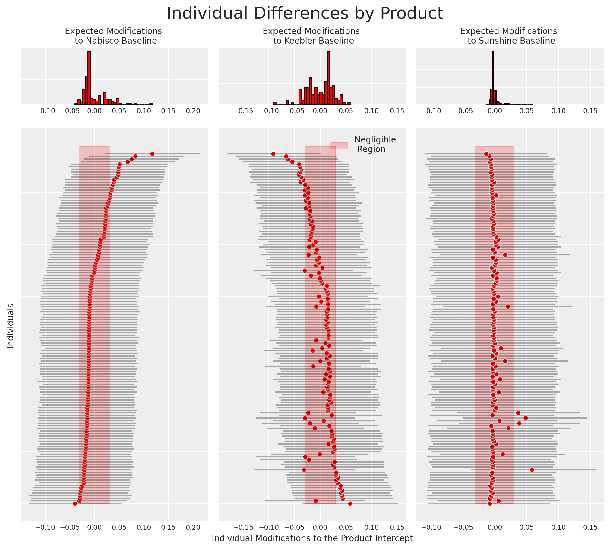
这种类型的图表通常有助于识别忠实客户。同样,它也可以用于识别应该更好地激励的客户群体,如果我们希望他们转向我们的产品。
结论#
我们可以在这里看到建模离散选项个体选择的灵活性和丰富参数化的可能性。这些技术在从微观经济学到市场营销和产品开发的广泛领域中都很有用。效用、概率及其相互作用的观念是Savage表示定理和贝叶斯统计推断的正当性(s)的核心。因此,离散建模自然适合贝叶斯,但贝叶斯统计也自然适合离散选择建模。传统的估计技术通常很脆弱,并且非常依赖于MLE过程的初始值。贝叶斯框架用这种脆弱性换取了一个允许我们结合我们对驱动人类效用计算的因素的信念的框架。在这个示例笔记本中,我们只是触及了表面,但我们鼓励您进一步探索这项技术。
参考资料#
水印#
%load_ext watermark
%watermark -n -u -v -iv -w -p pytensor
Last updated: Thu Jul 13 2023

Python implementation: CPython
Python version       : 3.9.16
IPython version      : 8.11.0

pytensor: 2.11.1

numpy     : 1.23.5
matplotlib: 3.7.1
pytensor  : 2.11.1
pandas    : 1.5.3
arviz     : 0.15.1
pymc      : 5.3.0

Watermark: 2.3.1