脆弱性和生存回归模型

import os

import arviz as az
import matplotlib.pyplot as plt
import numpy as np
import pandas as pd
import pymc as pm
import pytensor.tensor as pt

from lifelines import KaplanMeierFitter
from matplotlib import cm
from matplotlib.lines import Line2D
from scipy.stats import fisk, weibull_min

%config InlineBackend.figure_format = 'retina'  # high resolution figures
az.style.use("arviz-darkgrid")
rng = np.random.default_rng(42)

生存分析的全部普遍性和应用范围被医学术语的繁重语义所掩盖。在跨越日历和里程碑的生活中，自我关注的持续焦虑掩盖了这一点。但广义上的生存分析并不是关于你，它甚至不一定与生存有关。

从医学背景转向认识到时间到事件数据无处不在，需要一个额外的抽象步骤！每个具有隐含时钟的任务，每个有终点的目标，每个应支付费用的收割者——这些都是时间到事件数据的来源。

我们将演示如何将基于生存的回归分析概念（传统上应用于医疗环境）有效地应用于人力资源数据和业务流程分析。特别是，我们将探讨员工生命周期数据中的离职时间问题，并将其建模为员工在年初记录的调查响应的函数。

生存回归模型

这里的重点是框架的通用性。我们正在描述状态转换在时间内的轨迹。在任何速度或效率重要的地方，理解时间到事件轨迹的输入都很重要。这就是生存分析的好处——清晰阐述的模型，量化了人口特征和治疗效果（在速度方面）对状态转换概率的影响。从生到死、从雇佣到解雇、从生病到治愈、从订阅到流失。这些状态转换都使用生存回归模型进行了透明且有说服力的建模。

我们将看到两种针对时间到事件数据的回归建模方法：(1) Cox比例风险模型和(2) 加速失效时间模型。这两种模型都使分析师能够结合并评估不同协变量对生存时间结果的影响，但每种模型在处理方式上略有不同。

我们还将展示一种称为脆弱性建模的分层生存模型变体，其中我们使用回归来估计生存函数，但允许包含个体或群体特定的“脆弱性”项。这些是应用于个体生存曲线估计程序的乘法因子，使我们能够捕捉到人群中一些无法解释的异质性。此外，我们还将展示如何表达分层方法来估计基线风险。在整个过程中，我们将参考Collett [2014]中的讨论。

数据探索

人员分析本质上是对业务中的效率和风险的理解——生存分析特别适合阐明这两个问题。我们的示例数据来自Keith McNulty的《人员分析中的回归建模手册》中讨论的一个以人力资源为主题的案例 McKnulty [2020]。

数据描述了关于工作满意度和受访者是否有意向在其他地方寻找工作的调查问卷回复。此外，数据还包括受访者的广泛“人口统计”信息，以及关键的指示，表明他们是否离职了公司，以及在调查后我们仍然有记录的月份。我们希望了解随着时间的推移，员工流失的概率作为员工调查回复的函数，以帮助（a）管理因人手不足而带来的风险，以及（b）通过维持适当的人员配置来确保效率。

需要注意的是，这种数据总是截断数据，因为它总是在某个时间点提取的。因此，对于某些人，我们没有看到离职事件。他们可能永远不会离开公司——但重要的是，在测量时，我们根本不知道他们明天是否会离开……因此，数据在测量时是有意义地截断的。我们的建模策略需要考虑这一点，因为它会改变所讨论的概率，如贝叶斯回归与截断或截断数据中所讨论的。

try:
    retention_df = pd.read_csv(os.path.join("..", "data", "time_to_attrition.csv"))
except FileNotFoundError:
    retention_df = pd.read_csv(pm.get_data("time_to_attrition.csv"))


dummies = pd.concat(
    [
        pd.get_dummies(retention_df["gender"], drop_first=True),
        pd.get_dummies(retention_df["level"], drop_first=True),
        pd.get_dummies(retention_df["field"], drop_first=True),
    ],
    axis=1,
).rename({"M": "Male"}, axis=1)

retention_df = pd.concat([retention_df, dummies], axis=1).sort_values("Male").reset_index(drop=True)
retention_df.head()

	gender	field	level	sentiment	intention	left	month	Male	Low	Medium	Finance	Health	Law	Public/Government	Sales/Marketing
0	F	Education and Training	Low	8	5	0	12	0	1	0	0	0	0	0	0
1	F	Education and Training	Medium	8	3	1	11	0	0	1	0	0	0	0	0
2	F	Education and Training	Low	10	7	1	9	0	1	0	0	0	0	0	0
3	F	Education and Training	High	8	2	0	12	0	0	0	0	0	0	0	0
4	F	Education and Training	Low	8	8	0	12	0	1	0	0	0	0	0	0

我们已为下面回归模型中使用的一些分类变量添加了虚拟编码。我们删除了第一个编码类，因为这样可以避免估计过程中的识别问题。此外，这意味着为每个指示变量估计的系数相对于被删除的“参考”类具有解释意义。

首先，我们将查看在我们数据上估计的生存函数的简单Kaplan Meier表示。生存函数量化了在给定时间之前事件未发生的概率，即在特定月份之前员工流失的概率。自然地，不同类型的风险特征会导致不同的生存函数。回归模型，通常情况下，有助于解析风险的性质，当风险特征过于复杂而难以简单表述时。

kmf = KaplanMeierFitter()
kmf.fit(retention_df["month"], event_observed=retention_df["left"])
kmf_hi = KaplanMeierFitter()
kmf_hi.fit(
    retention_df[retention_df["sentiment"] == 10]["month"],
    event_observed=retention_df[retention_df["sentiment"] == 10]["left"],
)
kmf_mid = KaplanMeierFitter()
kmf_mid.fit(
    retention_df[retention_df["sentiment"] == 5]["month"],
    event_observed=retention_df[retention_df["sentiment"] == 5]["left"],
)
kmf_low = KaplanMeierFitter()
kmf_low.fit(
    retention_df[retention_df["sentiment"] == 2]["month"],
    event_observed=retention_df[retention_df["sentiment"] == 2]["left"],
)

fig, axs = plt.subplots(1, 2, figsize=(20, 15))
axs = axs.flatten()
ax = axs[0]
for i in retention_df.sample(30).index[0:30]:
    temp = retention_df[retention_df.index == i]
    event = temp["left"].max() == 1
    level = temp["level"].unique()
    duration = temp["month"].max()
    color = np.where(level == "High", "red", np.where(level == "Medium", "slateblue", "grey"))
    ax.hlines(i, 0, duration, color=color)
    if event:
        ax.scatter(duration, i, color=color)
ax.set_title("Assorted Time to Attrition \n by Level", fontsize=20)
ax.set_yticklabels([])
from matplotlib.lines import Line2D

custom_lines = [
    Line2D([0], [0], color="red", lw=4),
    Line2D([0], [0], color="slateblue", lw=4),
    Line2D([0], [0], color="grey", lw=4),
]

ax.legend(custom_lines, ["High Sentiment", "Medium Sentiment", "Low Sentiment"])


kmf_hi.plot_survival_function(ax=axs[1], label="KM estimate for High Sentiment", color="red")
kmf_mid.plot_survival_function(
    ax=axs[1], label="KM estimate for Medium Sentiment", color="slateblue"
)
kmf_low.plot_survival_function(ax=axs[1], label="KM estimate for Low Sentiment", color="grey")
kmf.plot_survival_function(
    ax=axs[1], label="Overall KM estimate", color="cyan", at_risk_counts=True
)
axs[1].set_xlabel("Time in Months")
axs[1].set_title("Kaplan Meier Fits by Level", fontsize=20);

/Users/nathanielforde/mambaforge/envs/pymc_examples_new/lib/python3.9/site-packages/lifelines/plotting.py:964: UserWarning: The figure layout has changed to tight
  plt.tight_layout()

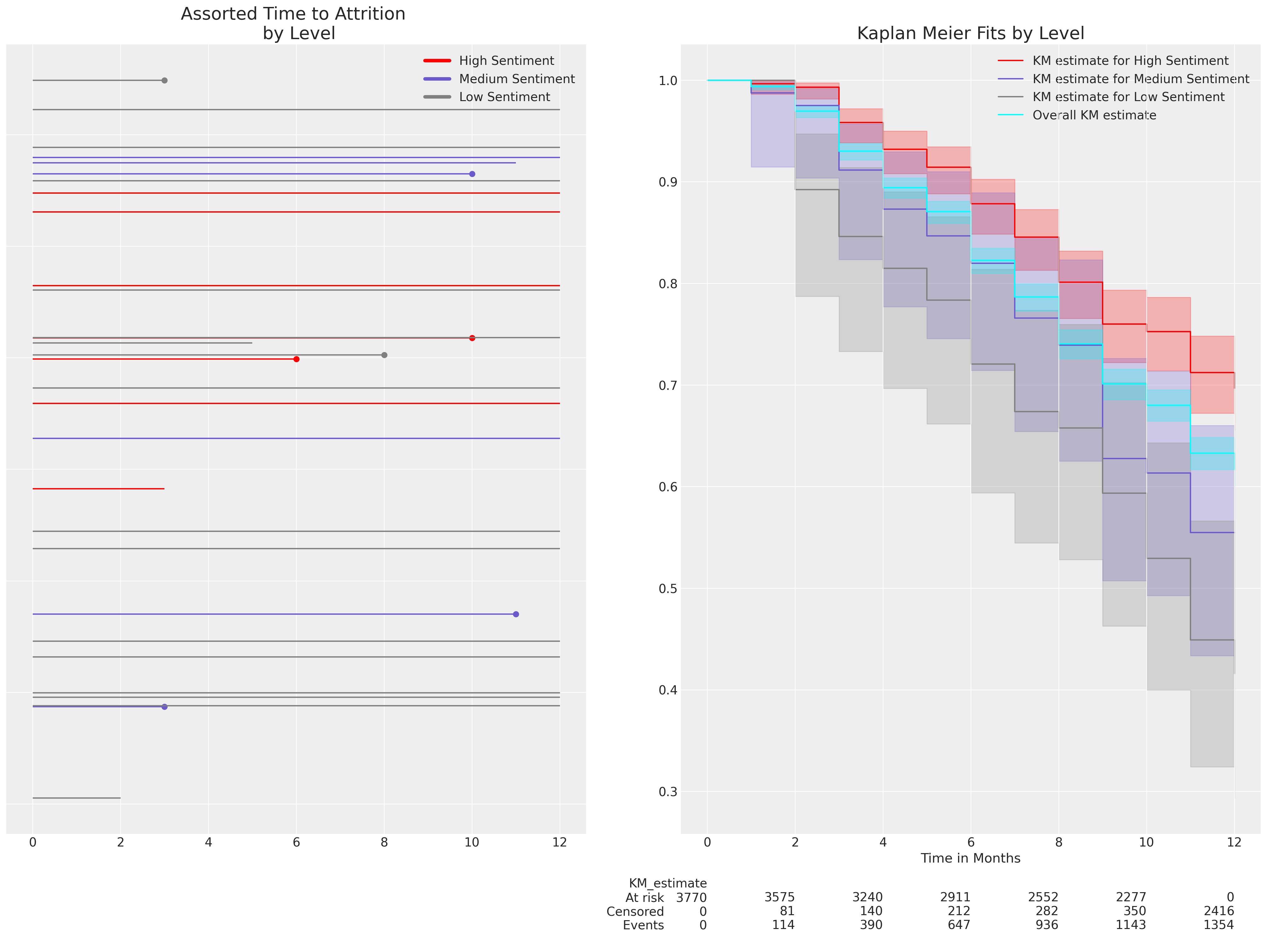
这里我们使用了Kaplan Meier非参数估计法来估计在sentiment变量不同水平下的生存曲线，以展示在试验期开始时参与者表达的sentiment水平如何影响12个月期间的预期流失水平。这只是对生存曲线的探索性数据分析，但我们希望了解概率模型如何恢复这些生存曲线以及概率模型的适当解释是什么。情绪越低，流失发生得越快。

生存回归的数据准备

Cox比例风险回归模型的核心思想，粗略地说，是认真对待风险的时序成分。我们设想一个潜在的基线风险，它在时间间隔内发生。Michael Betancourt 提出我们将风险视为“某种刺激资源的积累”，这种资源在事件发生之前积累。在故障建模中，它可以被想象为间歇性的磨损增加。在人力资源动态的背景下，它可以被想象为工作环境中日益增加的挫折感。在哲学中，它可以被视为堆垛悖论的一种表述；随着沙子堆得越来越高，我们如何识别一堆沙子，以及机会如何随着时间的推移而变化？这个术语通常表示为：

\[ \lambda_{0}(t)\]

它在Cox回归中与个体案例的线性协变量表示相结合：

\[ \lambda_{0}(t) \cdot exp(\beta_{1}X_{1} + \beta_{2}X_{2}... \beta_{k}X_{k}) \]

并表示在预测变量设置为其基线/参考水平时，每个时间点的基线风险。也就是说，回归模型中任何协变量\(X_{i}\)从0开始的任何单位增加都会改变基线风险。在我们的例子中，我们正在查看具有月度条目粒度的数据。因此，我们需要了解在年度调查日期之后的接下来12个月内，流失风险如何变化，以及每个个体的协变量概况如何改变基线风险。

这些模型可以使用Austin Rochford在贝叶斯生存分析中概述的贝叶斯估计方法进行估计。接下来，我们在他的示例基础上进行构建。首先，我们指定风险的时间维度，在我们的例子中，我们有一年内的每月间隔——表示自调查响应日期以来的时间。

intervals = np.arange(12)
intervals

array([ 0,  1,  2,  3,  4,  5,  6,  7,  8,  9, 10, 11])

然后，我们将数据整理成一个结构，以显示数据集中的每个个体是否以及何时经历了流失事件。这里的列表示每个月的指标，行表示数据集中的每个个体。值为1表示该员工在该月离职，否则为0。

n_employees = retention_df.shape[0]
n_intervals = len(intervals)
last_period = np.floor((retention_df.month - 0.01) / 1).astype(int)
employees = np.arange(n_employees)
quit = np.zeros((n_employees, n_intervals))
quit[employees, last_period] = retention_df["left"]

pd.DataFrame(quit)

	0	1	2	3	4	5	6	7	8	9	10	11
0	0.0	0.0	0.0	0.0	0.0	0.0	0.0	0.0	0.0	0.0	0.0	0.0
1	0.0	0.0	0.0	0.0	0.0	0.0	0.0	0.0	0.0	0.0	1.0	0.0
2	0.0	0.0	0.0	0.0	0.0	0.0	0.0	0.0	1.0	0.0	0.0	0.0
3	0.0	0.0	0.0	0.0	0.0	0.0	0.0	0.0	0.0	0.0	0.0	0.0
4	0.0	0.0	0.0	0.0	0.0	0.0	0.0	0.0	0.0	0.0	0.0	0.0
...	...	...	...	...	...	...	...	...	...	...	...	...
3765	0.0	0.0	1.0	0.0	0.0	0.0	0.0	0.0	0.0	0.0	0.0	0.0
3766	0.0	0.0	0.0	0.0	0.0	0.0	1.0	0.0	0.0	0.0	0.0	0.0
3767	0.0	0.0	0.0	0.0	0.0	0.0	0.0	0.0	0.0	0.0	0.0	0.0
3768	0.0	0.0	0.0	0.0	0.0	0.0	0.0	0.0	0.0	0.0	0.0	0.0
3769	0.0	0.0	0.0	0.0	0.0	0.0	0.0	0.0	0.0	0.0	0.0	0.0

3770 行 × 12 列

如可靠性统计与预测校准中所述，风险函数、累积密度函数和事件时间分布的生存函数都密切相关。特别是，这些函数中的每一个都可以根据在序列中任何给定时间处于风险中的个体集合来描述。随着人们经历流失事件，处于风险中的个体池会随着时间的推移而变化。这改变了随时间变化的条件风险——并对隐含的生存函数产生连锁影响。为了在我们的估计策略中考虑这一点，我们需要配置我们的数据以标记谁处于风险中以及何时处于风险中。

exposure = np.greater_equal.outer(retention_df.month.to_numpy(), intervals) * 1
exposure[employees, last_period] = retention_df.month - intervals[last_period]
pd.DataFrame(exposure)

	0	1	2	3	4	5	6	7	8	9	10	11
0	1	1	1	1	1	1	1	1	1	1	1	1
1	1	1	1	1	1	1	1	1	1	1	1	1
2	1	1	1	1	1	1	1	1	1	1	0	0
3	1	1	1	1	1	1	1	1	1	1	1	1
4	1	1	1	1	1	1	1	1	1	1	1	1
...	...	...	...	...	...	...	...	...	...	...	...	...
3765	1	1	1	1	0	0	0	0	0	0	0	0
3766	1	1	1	1	1	1	1	1	0	0	0	0
3767	1	1	1	1	1	1	1	1	1	1	1	1
3768	1	1	1	1	1	1	1	1	1	1	1	1
3769	1	1	1	1	1	1	1	1	1	1	1	1

3770 行 × 12 列

在此数据结构中，0 表示该员工已经离职，并且在当时的时间点不再存在于“风险”池中。而 1 则表示该员工在风险池中，应使用该值来计算该时间间隔内的瞬时风险。

通过这些结构，我们现在可以估计我们的模型。按照Austin Rochford的例子，我们再次使用泊松技巧来估计比例风险模型。这可能有些令人惊讶，因为Cox比例风险模型通常被宣传为一种半参数模型，由于基准风险分量的分段性质，需要使用部分似然法进行估计。

关键在于理解事件计数的泊松回归和CoxPH回归通过决定事件发生率的参数相互关联。在预测计数的情况下，我们需要一个潜在的事件风险，该风险通过每个时间间隔的偏移量来索引时间。这确保了泊松回归的似然项与Cox比例风险回归中考虑的似然项足够相似，从而可以用一个替代另一个。换句话说，Cox比例风险模型可以被估计为使用泊松似然的广义线性模型（GLM），其中我们为时间间隔上的每个点指定一个“偏移量”或截距修正。使用Wilkinson符号，我们可以写成：

\[ CoxPH(left, month) \sim gender + level \]

类似于

\[\begin{split} left \sim glm(gender + level + (1 | month)) \\ \text{ where link is } Poisson \end{split}\]

我们使用上述定义的结构和PyMC进行估计，如下所示：

拟合带有固定效应的基本Cox模型

我们将设置一个模型工厂函数，以适应具有不同协变量规范的基本Cox比例风险模型。我们希望评估测量离职意向的模型与不测量离职意向的模型之间的模型含义差异。

preds = [
    "sentiment",
    "Male",
    "Low",
    "Medium",
    "Finance",
    "Health",
    "Law",
    "Public/Government",
    "Sales/Marketing",
]
preds2 = [
    "sentiment",
    "intention",
    "Male",
    "Low",
    "Medium",
    "Finance",
    "Health",
    "Law",
    "Public/Government",
    "Sales/Marketing",
]


def make_coxph(preds):
    coords = {"intervals": intervals, "preds": preds, "individuals": range(len(retention_df))}

    with pm.Model(coords=coords) as base_model:
        X_data = pm.MutableData("X_data_obs", retention_df[preds], dims=("individuals", "preds"))
        lambda0 = pm.Gamma("lambda0", 0.01, 0.01, dims="intervals")

        beta = pm.Normal("beta", 0, sigma=1, dims="preds")
        lambda_ = pm.Deterministic(
            "lambda_",
            pt.outer(pt.exp(pm.math.dot(beta, X_data.T)), lambda0),
            dims=("individuals", "intervals"),
        )

        mu = pm.Deterministic("mu", exposure * lambda_, dims=("individuals", "intervals"))

        obs = pm.Poisson("obs", mu, observed=quit, dims=("individuals", "intervals"))
        base_idata = pm.sample(
            target_accept=0.95, random_seed=100, idata_kwargs={"log_likelihood": True}
        )

    return base_idata, base_model


base_idata, base_model = make_coxph(preds)
base_intention_idata, base_intention_model = make_coxph(preds2)

Auto-assigning NUTS sampler...
Initializing NUTS using jitter+adapt_diag...
Multiprocess sampling (4 chains in 4 jobs)
NUTS: [lambda0, beta]

100.00% [8000/8000 01:02<00:00 Sampling 4 chains, 0 divergences]

Sampling 4 chains for 1_000 tune and 1_000 draw iterations (4_000 + 4_000 draws total) took 62 seconds.
Auto-assigning NUTS sampler...
Initializing NUTS using jitter+adapt_diag...
Multiprocess sampling (4 chains in 4 jobs)
NUTS: [lambda0, beta]

100.00% [8000/8000 01:12<00:00 Sampling 4 chains, 0 divergences]

Sampling 4 chains for 1_000 tune and 1_000 draw iterations (4_000 + 4_000 draws total) took 72 seconds.

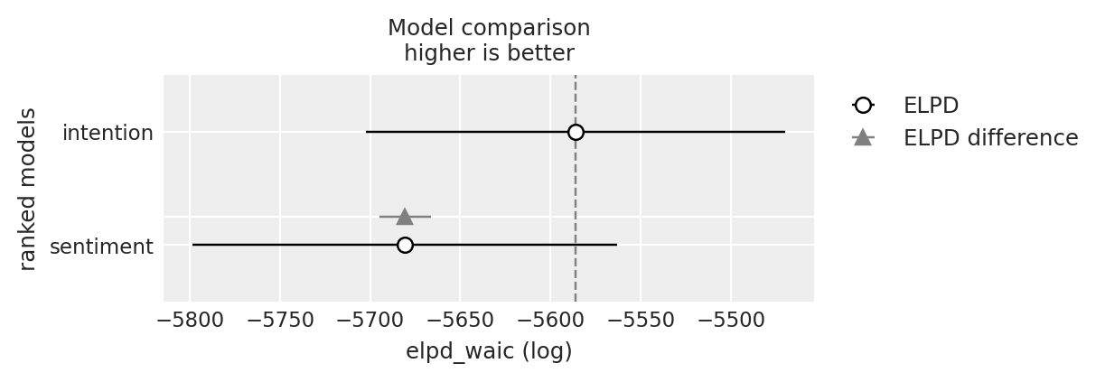
compare = az.compare({"sentiment": base_idata, "intention": base_intention_idata}, ic="waic")
compare

	rank	elpd_waic	p_waic	elpd_diff	weight	se	dse	warning	scale
intention	0	-5586.085248	21.327895	0.000000	0.996278	115.944586	0.000000	False	log
sentiment	1	-5680.561115	20.101640	94.475867	0.003722	117.596277	14.181559	False	log

az.plot_compare(compare);

pm.model_to_graphviz(base_model)

我们可以看到，模型的结构虽然与典型的回归模型略有不同，但包含了所有相同的元素。观察到的变量在加权和中结合，并向前传递以修改结果。在我们的例子中，结果是危险——或在特定时间点的条件风险。正是这一系列估计构成了我们对该时期风险演变性质的看法。那么一个明显的问题是，预测变量如何对风险的演变做出贡献。

一个次要问题是，实例层面的风险视图如何转化为随时间推移的生存概率视图？我们如何从基于风险的角度转变为基于生存的角度？

解释模型系数

我们将首先关注我们两个模型中输入变量的差异性影响。beta参数估计值记录在对数风险率尺度上。首先看看intention预测变量（一个衡量调查参与者戒烟意愿的分数）如何改变未包含此变量的模型中参数估计的大小和符号。这是一个简单但有力的提醒，确保我们测量正确的事物，并且进入我们模型的特征/变量是否构成关于数据生成过程的故事，无论我们是否关注。

m = (
    az.summary(base_idata, var_names=["beta"])
    .reset_index()[["index", "mean"]]
    .rename({"mean": "expected_hr"}, axis=1)
)
m1 = (
    az.summary(base_intention_idata, var_names=["beta"])
    .reset_index()[["index", "mean"]]
    .rename({"mean": "expected_intention_hr"}, axis=1)
)
m = m.merge(m1, left_on="index", right_on="index", how="outer")
m["exp(expected_hr)"] = np.exp(m["expected_hr"])
m["exp(expected_intention_hr)"] = np.exp(m["expected_intention_hr"])
m

	index	expected_hr	expected_intention_hr	exp(expected_hr)	exp(expected_intention_hr)
0	beta[sentiment]	-0.110	-0.029	0.895834	0.971416
1	beta[Male]	-0.037	0.015	0.963676	1.015113
2	beta[Low]	0.137	0.155	1.146828	1.167658
3	beta[Medium]	0.161	0.107	1.174685	1.112934
4	beta[Finance]	0.207	0.234	1.229983	1.263644
5	beta[Health]	0.249	0.236	1.282742	1.266174
6	beta[Law]	0.091	0.073	1.095269	1.075731
7	beta[Public/Government]	0.102	0.120	1.107383	1.127497
8	beta[Sales/Marketing]	0.075	0.100	1.077884	1.105171
9	beta[intention]	NaN	0.189	NaN	1.208041

每个单独的模型系数记录了输入变量每增加一个单位对对数风险比的影响估计。请注意，我们是如何对系数进行指数运算以将其恢复到风险比的比例的。对于具有系数 \(\beta\) 的预测变量 \(X\)，解释如下：

• 如果 \(exp(\beta)\) 大于 1：X 的增加与事件发生的风险（危险）增加相关。

• 如果 \(exp(\beta)\) < 1：X 的增加与事件发生的风险降低（较低的风险）相关。

• 如果 \(exp(\beta)\) = 1：X 对危险率没有影响。

因此，在我们的案例中，我们可以看到，在金融或健康领域拥有职业似乎会使事件发生的风险比基线风险增加约25%。有趣的是，我们可以看到，包含intention预测因子似乎很重要，因为intention指标的单位增加同样会移动刻度盘——而intention是一个0-10的刻度。

这些不是随时间变化的——它们在加权和中一次进入，以修改基线风险。这是比例风险假设——即尽管基线风险可能随时间变化，但由协变量不同水平引起的风险差异在时间上是恒定的。Cox模型之所以流行，是因为它允许我们在每个时间点估计变化的风险，并将人口统计预测因子的影响在整个时间段内乘法地结合起来。比例风险假设并不总是成立，我们将在下面看到一些调整方法，这些方法可以帮助处理比例风险假设的违反情况。

fig, ax = plt.subplots(figsize=(20, 6))
ax.plot(base_idata["posterior"]["lambda0"].mean(("draw", "chain")), color="black")
az.plot_hdi(
    range(12),
    base_idata["posterior"]["lambda0"],
    color="lightblue",
    ax=ax,
    hdi_prob=0.99,
    fill_kwargs={"label": "Baseline Hazard 99%", "alpha": 0.3},
    smooth=False,
)
az.plot_hdi(
    range(12),
    base_idata["posterior"]["lambda0"],
    color="lightblue",
    ax=ax,
    hdi_prob=0.50,
    fill_kwargs={"label": "Baseline Hazard 50%", "alpha": 0.8},
    smooth=False,
)
ax.legend()
ax.set_xlabel("Time")
ax.set_title("Expected Baseline Hazard", fontsize=20);

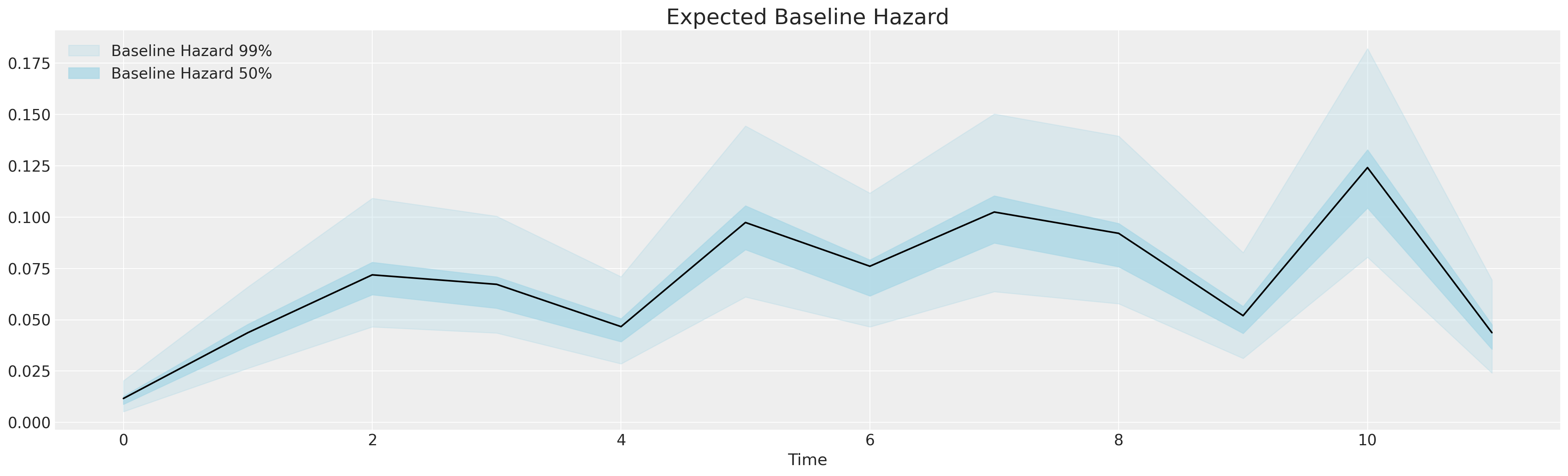
这是基线刺激 - 不断增长、间歇性变化的危险因素，促使磨损的发生。我们构建了包含一系列控制变量和处理指示符的回归模型，以评估它们在随时间改变基线危险方面的任何影响。生存回归建模是一种透明的工具，用于分析人口统计和行为特征对风险随时间变化的影响。注意在年度周期结束时的急剧增加。

预测CoxPH回归的边际效应

我们可以通过推导样本/虚构数据上的边际效应，使这些解释更加具体。现在我们定义生存与累积危险度量之间的关系作为基线危险的函数。

def cum_hazard(hazard):
    """Takes arviz.InferenceData object applies
    cumulative sum along baseline hazard"""
    return hazard.cumsum(dim="intervals")


def survival(hazard):
    """Takes arviz.InferenceData object transforms
    cumulative hazard into survival function"""
    return np.exp(-cum_hazard(hazard))


def get_mean(trace):
    """Takes arviz.InferenceData object marginalises
    over the chain and draw"""
    return trace.mean(("draw", "chain"))

累积风险函数平滑了基础风险函数的跳跃性，使我们能够更清晰地了解随着时间推移风险增加的程度。这进而转化为我们的生存函数，该函数很好地在0-1尺度上表达了风险。接下来，我们设置一个函数来推导每个个体在其风险特征条件下的生存函数和累积风险函数。

def extract_individual_hazard(idata, i, retention_df, intention=False):
    beta = idata.posterior["beta"]
    if intention:
        intention_posterior = beta.sel(preds="intention")
    else:
        intention_posterior = 0
    hazard_base_m1 = idata["posterior"]["lambda0"]

    full_hazard_idata = hazard_base_m1 * np.exp(
        beta.sel(preds="sentiment") * retention_df.iloc[i]["sentiment"]
        + np.where(intention, intention_posterior * retention_df.iloc[i]["intention"], 0)
        + beta.sel(preds="Male") * retention_df.iloc[i]["Male"]
        + beta.sel(preds="Low") * retention_df.iloc[i]["Low"]
        + beta.sel(preds="Medium") * retention_df.iloc[i]["Medium"]
        + beta.sel(preds="Finance") * retention_df.iloc[i]["Finance"]
        + beta.sel(preds="Health") * retention_df.iloc[i]["Health"]
        + beta.sel(preds="Law") * retention_df.iloc[i]["Law"]
        + beta.sel(preds="Public/Government") * retention_df.iloc[i]["Public/Government"]
        + beta.sel(preds="Sales/Marketing") * retention_df.iloc[i]["Sales/Marketing"]
    )

    cum_haz_idata = cum_hazard(full_hazard_idata)
    survival_idata = survival(full_hazard_idata)
    return full_hazard_idata, cum_haz_idata, survival_idata, hazard_base_m1


def plot_individuals(retention_df, idata, individuals=[1, 300, 700], intention=False):
    fig, axs = plt.subplots(1, 2, figsize=(20, 7))
    axs = axs.flatten()
    colors = ["slateblue", "magenta", "darkgreen"]
    for i, c in zip(individuals, colors):
        haz_idata, cum_haz_idata, survival_idata, base_hazard = extract_individual_hazard(
            idata, i, retention_df, intention
        )
        axs[0].plot(get_mean(survival_idata), label=f"individual_{i}", color=c)
        az.plot_hdi(range(12), survival_idata, ax=axs[0], fill_kwargs={"color": c})
        axs[1].plot(get_mean(cum_haz_idata), label=f"individual_{i}", color=c)
        az.plot_hdi(range(12), cum_haz_idata, ax=axs[1], fill_kwargs={"color": c})
        axs[0].set_title("Individual Survival Functions", fontsize=20)
        axs[1].set_title("Individual Cumulative Hazard Functions", fontsize=20)
    az.plot_hdi(
        range(12),
        survival(base_hazard),
        color="lightblue",
        ax=axs[0],
        fill_kwargs={"label": "Baseline Survival"},
    )
    axs[0].plot(
        get_mean(survival(base_hazard)),
        color="black",
        linestyle="--",
        label="Expected Baseline Survival",
    )
    az.plot_hdi(
        range(12),
        cum_hazard(base_hazard),
        color="lightblue",
        ax=axs[1],
        fill_kwargs={"label": "Baseline Hazard"},
    )
    axs[1].plot(
        get_mean(cum_hazard(base_hazard)),
        color="black",
        linestyle="--",
        label="Expected Baseline Hazard",
    )
    axs[0].legend()
    axs[0].set_ylabel("Probability of Survival")
    axs[1].set_ylabel("Cumulative Hazard Risk")
    axs[0].set_xlabel("Time")
    axs[1].set_xlabel("Time")
    axs[1].legend()


#### Next set up test-data input to explore the relationship between levels of the variables.
test_df = pd.DataFrame(np.zeros((3, 15)), columns=retention_df.columns)
test_df["sentiment"] = [1, 5, 10]
test_df["intention"] = [1, 5, 10]
test_df["Medium"] = [0, 0, 0]
test_df["Finance"] = [0, 0, 0]
test_df["M"] = [1, 1, 1]
test_df

	gender	field	level	sentiment	intention	left	month	Male	Low	Medium	Finance	Health	Law	Public/Government	Sales/Marketing	M
0	0.0	0.0	0.0	1	1	0.0	0.0	0.0	0.0	0	0	0.0	0.0	0.0	0.0	1
1	0.0	0.0	0.0	5	5	0.0	0.0	0.0	0.0	0	0	0.0	0.0	0.0	0.0	1
2	0.0	0.0	0.0	10	10	0.0	0.0	0.0	0.0	0	0	0.0	0.0	0.0	0.0	1

意图模型

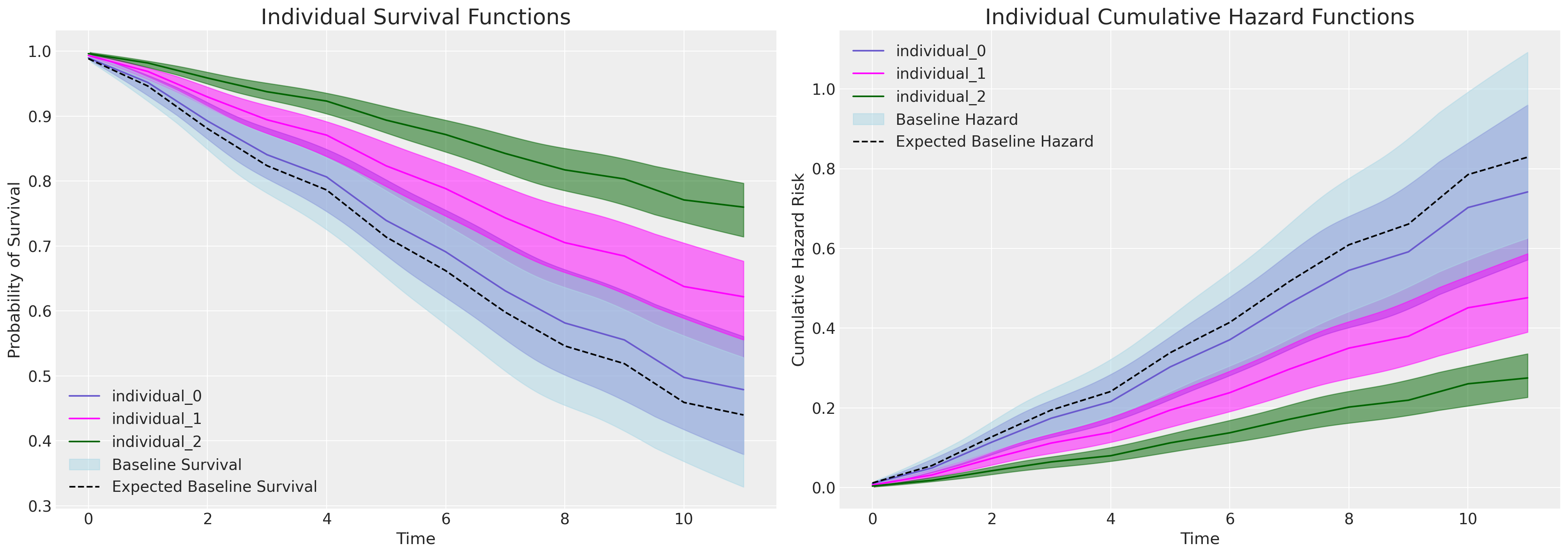
如果我们绘制由于intention变量增加而产生的边际效应——在能够评估它的模型中，我们会看到个体预测生存曲线中明显的分界线，这与上述系数表中intention变量的显著且重要的参数估计相符。

plot_individuals(test_df, base_intention_idata, [0, 1, 2], intention=True)

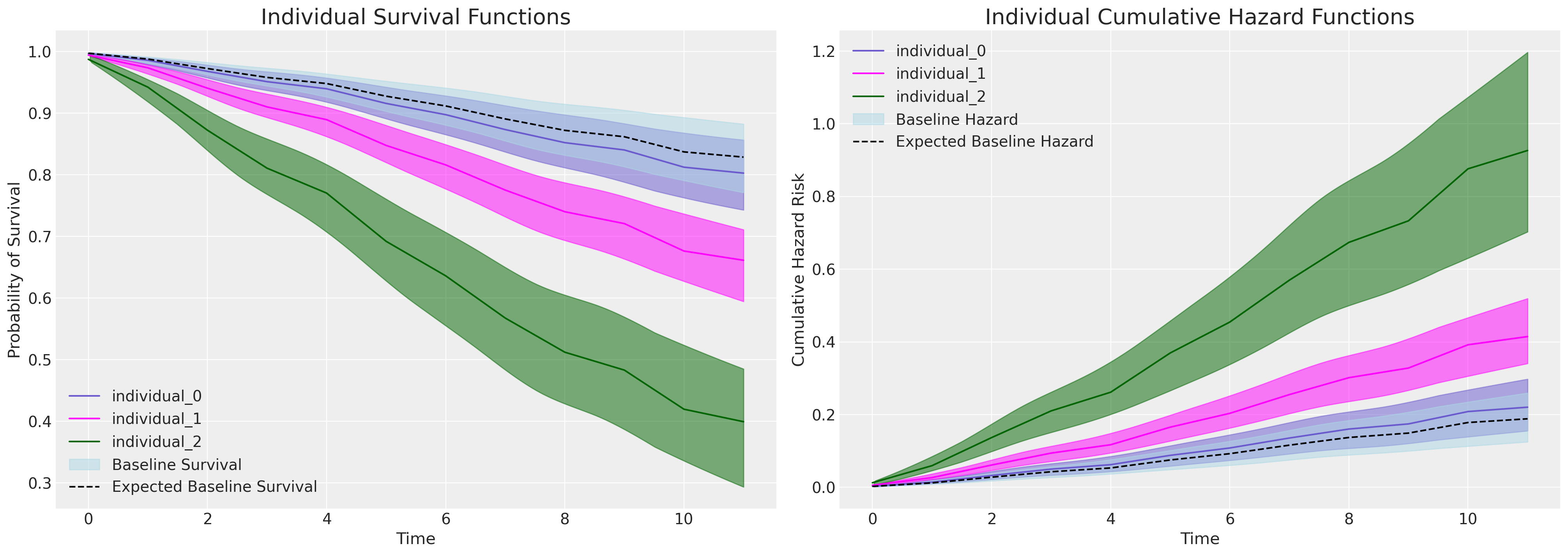
请关注右侧的图表。基线累积风险以蓝色表示，随后的每条曲线代表在intention指标上得分增加的个体的累积风险，即风险增加。这种模式在左侧的图表中是相反的——在这里，我们看到的是随着时间的推移，具有高intention值的个体的生存概率下降得更为急剧。

情感模型

如果我们向一个无法考虑意图的模型提交相同的测试，大部分权重会落在调查参与者记录的情感之间的差异上。在这里，我们也可以看到生存曲线的分离，但效果要小得多。

plot_individuals(test_df, base_idata, [0, 1, 2], intention=False)

这里需要注意的一个重要观察结果是，每个模型中基线风险做了多少工作。在可以考虑意图指标影响的模型中，基线风险较低。这表明基线风险需要做更多的工作。其他测试数据和输入规范的组合可以用来以这种方式实验CoxPh模型的条件影响。

为个体特征进行预测

使用边际效应分析来更好地理解特定变量的影响固然很好，但我们如何利用它来预测我们调查员工中的可能轨迹呢？在这里，我们只需将模型重新应用于我们的观察数据集，其中每个参与者在某种程度上由我们模型的可观察输入来表征。

我们可以利用这些特征来预测我们现有或未来员工群体的生存曲线，并在必要时进行干预，以减轻这些员工风险特征和类似员工风险特征的离职风险。

def create_predictions(retention_df, idata, intention=False):
    cum_haz = {}
    surv = {}
    for i in range(len(retention_df)):
        haz_idata, cum_haz_idata, survival_idata, base_hazard = extract_individual_hazard(
            idata, i, retention_df, intention=intention
        )
        cum_haz[i] = get_mean(cum_haz_idata)
        surv[i] = get_mean(survival_idata)
    cum_haz = pd.DataFrame(cum_haz)
    surv = pd.DataFrame(surv)
    return cum_haz, surv


cum_haz_df, surv_df = create_predictions(retention_df, base_idata, intention=False)
surv_df

	0	1	2	3	4	5	6	7	8	9	...	3760	3761	3762	3763	3764	3765	3766	3767	3768	3769
0	0.994518	0.994380	0.995593	0.995206	0.994518	0.994583	0.994518	0.990579	0.992487	0.992931	...	0.992586	0.993310	0.988610	0.995757	0.995011	0.992717	0.993964	0.993364	0.993472	0.994148
1	0.974209	0.973561	0.979227	0.977416	0.974209	0.974516	0.974209	0.956012	0.964789	0.966834	...	0.965227	0.968581	0.946990	0.979984	0.976493	0.965843	0.971611	0.968831	0.969341	0.972481
2	0.941695	0.940254	0.952883	0.948839	0.941695	0.942373	0.941695	0.901768	0.920887	0.925422	...	0.921831	0.929225	0.882325	0.954570	0.946789	0.923202	0.935920	0.929808	0.930906	0.937853
3	0.912256	0.910122	0.928877	0.922866	0.912256	0.913260	0.912256	0.853823	0.881618	0.888305	...	0.883002	0.893866	0.825868	0.931396	0.919829	0.885028	0.903721	0.894759	0.896340	0.906584
4	0.892383	0.889804	0.912586	0.905277	0.892383	0.893598	0.892383	0.822082	0.855371	0.863449	...	0.857049	0.870148	0.788869	0.915657	0.901596	0.859485	0.882054	0.871244	0.873125	0.885513
5	0.852282	0.848839	0.879493	0.869634	0.852282	0.853915	0.852282	0.759607	0.803079	0.813822	...	0.805304	0.822650	0.716938	0.883650	0.864693	0.808524	0.838480	0.824164	0.826588	0.843096
6	0.822221	0.818154	0.854484	0.842780	0.822221	0.824154	0.822221	0.714154	0.764475	0.777070	...	0.767064	0.787359	0.665387	0.859430	0.836926	0.770838	0.805941	0.789185	0.791977	0.811387
7	0.783397	0.778581	0.821918	0.807920	0.783397	0.785703	0.783397	0.657223	0.715395	0.730204	...	0.718425	0.742221	0.601809	0.827853	0.800941	0.722843	0.764111	0.744436	0.747639	0.770556
8	0.750084	0.744669	0.793722	0.777839	0.750084	0.752690	0.750084	0.609981	0.673991	0.690544	...	0.677365	0.703892	0.549930	0.800474	0.769951	0.682285	0.728390	0.706434	0.709932	0.735632
9	0.731908	0.726186	0.778234	0.761359	0.731908	0.734672	0.731908	0.584842	0.651689	0.669128	...	0.655238	0.683145	0.522666	0.785421	0.752995	0.660411	0.708973	0.685863	0.689499	0.716627
10	0.690271	0.683889	0.742464	0.723420	0.690271	0.693378	0.690271	0.528948	0.601379	0.620680	...	0.605290	0.636053	0.462957	0.750615	0.714028	0.610981	0.664683	0.639185	0.643059	0.673210
11	0.676189	0.669604	0.730273	0.710527	0.676189	0.679408	0.676189	0.510585	0.584615	0.604485	...	0.588636	0.620269	0.443621	0.738737	0.700803	0.594481	0.649766	0.623532	0.627471	0.658565

12 行 × 3770 列

样本生存曲线及其边际预期生存轨迹。

我们现在绘制这些个体风险概况，并对预测的生存曲线进行边际化处理。

cm_subsection = np.linspace(0, 1, 120)
colors_m = [cm.Purples(x) for x in cm_subsection]
colors = [cm.spring(x) for x in cm_subsection]


fig, axs = plt.subplots(1, 2, figsize=(20, 7))
axs = axs.flatten()
cum_haz_df.plot(legend=False, color=colors, alpha=0.05, ax=axs[1])
axs[1].plot(cum_haz_df.mean(axis=1), color="black", linewidth=4)
axs[1].set_title(
    "Individual Cumulative Hazard \n & Marginal Expected Cumulative Hazard", fontsize=20
)

surv_df.plot(legend=False, color=colors_m, alpha=0.05, ax=axs[0])
axs[0].plot(surv_df.mean(axis=1), color="black", linewidth=4)
axs[0].set_title("Individual Survival Curves \n  & Marginal Expected Survival Curve", fontsize=20)
axs[0].annotate(
    f"Expected Attrition by 6 months: {100*np.round(1-surv_df.mean(axis=1).iloc[6], 2)}%",
    (2, 0.5),
    fontsize=14,
    fontweight="bold",
);

这里的边际生存曲线是一个汇总统计量，就像在更简单的情况下测量平均值一样。它是样本数据（样本中的个体）的特征，因此你应该仅在满意地认为样本数据在比例上代表了总体中不同风险特征的情况下，将其视为一个指示性或可推广的度量。生存建模不是良好实验设计的替代品，但它可以用于分析实验数据。

在人力资源背景下，我们可能对管理培训计划影响下的员工流失时间指标感兴趣，或者在采用敏捷实践或新工具的软件开发团队中，对生产代码的提前期感兴趣。理解影响效率的政策是好的，理解政策影响效率的速度则更好。

加速失效时间模型

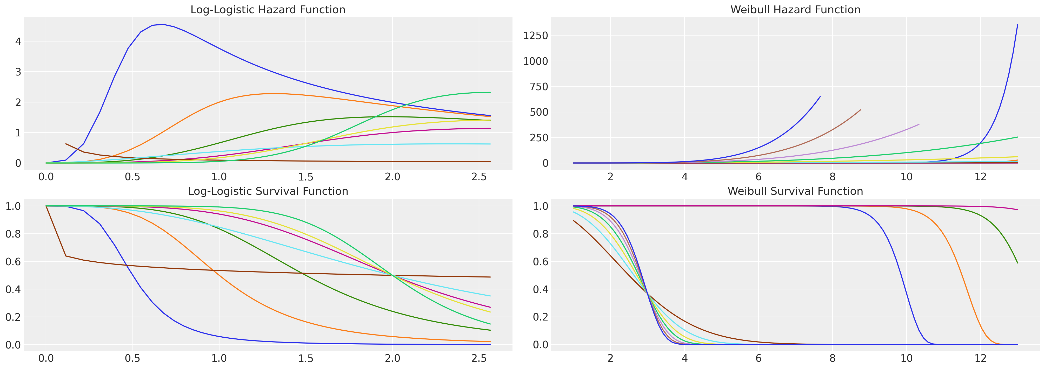
接下来我们研究一类基于回归的生存模型，称为加速失效时间模型（AFTs）。这些是回归模型，旨在通过引用一个或另一个可以用一组位置和尺度参数简洁描述的典型统计分布来描述感兴趣的生存函数，例如Weilbull分布、Log-Logistic分布和LogNormal分布等。这类分布的一个优点是，我们可以在不显式参数化时间间隔的情况下获得更灵活的 hazard 函数。

参见此处示例，了解对数逻辑分布如何表现出非单调的危险函数，而威布尔危险函数必然是单调的。如果你的案例理论允许事件发生风险的上升和下降，这是一个重要的观察结果。

fig, axs = plt.subplots(2, 2, figsize=(20, 7))
axs = axs.flatten()


def make_loglog_haz(alpha, beta):
    ## This is the Log Logistic distribution
    dist = fisk(c=alpha, scale=beta)
    t = np.log(np.linspace(1, 13, 100))  # Time values
    pdf_values = dist.pdf(t)
    sf_values = dist.sf(t)
    haz_values = pdf_values / sf_values
    axs[0].plot(t, haz_values)
    axs[2].plot(t, sf_values)


def make_weibull_haz(alpha, beta):
    dist = weibull_min(c=alpha, scale=beta)
    t = np.linspace(1, 13, 100)  # Time values
    pdf_values = dist.pdf(t)
    sf_values = dist.sf(t)
    haz_values = pdf_values / sf_values
    axs[1].plot(t, haz_values)
    axs[3].plot(t, sf_values)


[make_loglog_haz(4, b) for b in np.linspace(0.5, 2, 4)]
[make_loglog_haz(a, 2) for a in np.linspace(0.2, 7, 4)]
[make_weibull_haz(25, b) for b in np.linspace(10, 15, 4)]
[make_weibull_haz(a, 3) for a in np.linspace(2, 7, 7)]
axs[0].set_title("Log-Logistic Hazard Function", fontsize=15)
axs[2].set_title("Log-Logistic Survival Function", fontsize=15)
axs[1].set_title("Weibull Hazard Function", fontsize=15)
axs[3].set_title("Weibull Survival Function", fontsize=15);

AFT模型在回归模型中结合了解释变量，使得它们在时间尺度上乘性地作用，从而影响个体沿时间轴前进的速度。因此，该模型可以直接解释为通过感兴趣事件进展速度参数化的模型。AFT模型的生存函数通常指定为：

\[ S_{i}(t) = S_{0}\Bigg(\frac{t}{exp(\alpha_{i}x_{i} + \alpha_{2}x_{2} ... \alpha_{p}x_{p})} \Bigg) \]

其中 \(S_{0}\) 是基线生存率，但模型通常以对数线性形式表示：

\[ log (T_{i}) = \mu + \alpha_{i}x_{i} + \alpha_{2}x_{2} ... \alpha_{p}x_{p} + \sigma\epsilon_{i} \]

我们有一个基线生存函数 \(S_{0} = P(exp(\mu + \sigma\epsilon_{i}) \geq t)\)，它通过额外的协变量进行了修改。这些细节对于估计策略来说非常重要，但它们展示了如何在这里像在CoxPH模型中一样分解风险的影响。协变量的效应在个体风险概况引起的加速因子的对数尺度上是相加的。

下面我们将估计两个AFT模型：Weibull模型和Log-Logistic模型。最终我们只是拟合了一个截尾的参数分布，但我们允许每个分布的一个参数被指定为解释变量的线性函数。因此，对数似然项就是：

\[ log(L) = \sum_{i}^{n} \Big[ c_{i}log(f(t)) + (1-c_{i})log(S(t))) \Big] \]

其中 \(f\) 是分布的pdf函数，\(S\) 是生存函数，\(c\) 是一个指示函数，用于表示观察是否被删失——这意味着它取值于 \(\{0, 1\}\)，取决于个体是否被删失。\(f\) 和 \(S\) 都由某个参数向量 \(\mathbf{\theta}\) 参数化。在Log-Logistic模型的情况下，我们通过将时间变量转换为对数尺度并拟合具有参数 \(\mu, s\) 的逻辑似然来估计它。生成的参数拟合可以适应以恢复log-logistic生存函数，如下所示。在Weibull模型的情况下，参数分别表示为 \(\alpha, \beta\)。

coords = {
    "intervals": intervals,
    "preds": [
        "sentiment",
        "intention",
        "Male",
        "Low",
        "Medium",
        "Finance",
        "Health",
        "Law",
        "Public/Government",
        "Sales/Marketing",
    ],
}

X = retention_df[
    [
        "sentiment",
        "intention",
        "Male",
        "Low",
        "Medium",
        "Finance",
        "Health",
        "Law",
        "Public/Government",
        "Sales/Marketing",
    ]
].copy()
y = retention_df["month"].values
cens = retention_df.left.values == 0.0


def logistic_sf(y, μ, s):
    return 1.0 - pm.math.sigmoid((y - μ) / s)


def weibull_lccdf(x, alpha, beta):
    """Log complementary cdf of Weibull distribution."""
    return -((x / beta) ** alpha)


def make_aft(y, weibull=True):
    with pm.Model(coords=coords, check_bounds=False) as aft_model:
        X_data = pm.MutableData("X_data_obs", X)
        beta = pm.Normal("beta", 0.0, 1, dims="preds")
        mu = pm.Normal("mu", 0, 1)

        if weibull:
            s = pm.HalfNormal("s", 5.0)
            eta = pm.Deterministic("eta", pm.math.dot(beta, X_data.T))
            reg = pm.Deterministic("reg", pt.exp(-(mu + eta) / s))
            y_obs = pm.Weibull("y_obs", beta=reg[~cens], alpha=s, observed=y[~cens])
            y_cens = pm.Potential("y_cens", weibull_lccdf(y[cens], alpha=s, beta=reg[cens]))
        else:
            s = pm.HalfNormal("s", 5.0)
            eta = pm.Deterministic("eta", pm.math.dot(beta, X_data.T))
            reg = pm.Deterministic("reg", mu + eta)
            y_obs = pm.Logistic("y_obs", mu=reg[~cens], s=s, observed=y[~cens])
            y_cens = pm.Potential("y_cens", logistic_sf(y[cens], reg[cens], s=s))

        idata = pm.sample_prior_predictive()
        idata.extend(
            pm.sample(target_accept=0.95, random_seed=100, idata_kwargs={"log_likelihood": True})
        )
        idata.extend(pm.sample_posterior_predictive(idata))
    return idata, aft_model


weibull_idata, weibull_aft = make_aft(y)
## Log y to ensure we're estimating a log-logistic random variable
loglogistic_idata, loglogistic_aft = make_aft(np.log(y), weibull=False)

/var/folders/__/ng_3_9pn1f11ftyml_qr69vh0000gn/T/ipykernel_48265/3743381411.py:63: UserWarning: The effect of Potentials on other parameters is ignored during prior predictive sampling. This is likely to lead to invalid or biased predictive samples.
  idata = pm.sample_prior_predictive()
Sampling: [beta, mu, s, y_obs]
Auto-assigning NUTS sampler...
Initializing NUTS using jitter+adapt_diag...
Multiprocess sampling (4 chains in 4 jobs)
NUTS: [beta, mu, s]

100.00% [8000/8000 01:31<00:00 Sampling 4 chains, 0 divergences]

Sampling 4 chains for 1_000 tune and 1_000 draw iterations (4_000 + 4_000 draws total) took 91 seconds.
/var/folders/__/ng_3_9pn1f11ftyml_qr69vh0000gn/T/ipykernel_48265/3743381411.py:67: UserWarning: The effect of Potentials on other parameters is ignored during posterior predictive sampling. This is likely to lead to invalid or biased predictive samples.
  idata.extend(pm.sample_posterior_predictive(idata))
Sampling: [y_obs]

100.00% [4000/4000 00:00<00:00]

/var/folders/__/ng_3_9pn1f11ftyml_qr69vh0000gn/T/ipykernel_48265/3743381411.py:63: UserWarning: The effect of Potentials on other parameters is ignored during prior predictive sampling. This is likely to lead to invalid or biased predictive samples.
  idata = pm.sample_prior_predictive()
Sampling: [beta, mu, s, y_obs]
Auto-assigning NUTS sampler...
Initializing NUTS using jitter+adapt_diag...
Multiprocess sampling (4 chains in 4 jobs)
NUTS: [beta, mu, s]

100.00% [8000/8000 01:07<00:00 Sampling 4 chains, 0 divergences]

Sampling 4 chains for 1_000 tune and 1_000 draw iterations (4_000 + 4_000 draws total) took 67 seconds.
/var/folders/__/ng_3_9pn1f11ftyml_qr69vh0000gn/T/ipykernel_48265/3743381411.py:67: UserWarning: The effect of Potentials on other parameters is ignored during posterior predictive sampling. This is likely to lead to invalid or biased predictive samples.
  idata.extend(pm.sample_posterior_predictive(idata))
Sampling: [y_obs]

100.00% [4000/4000 00:00<00:00]

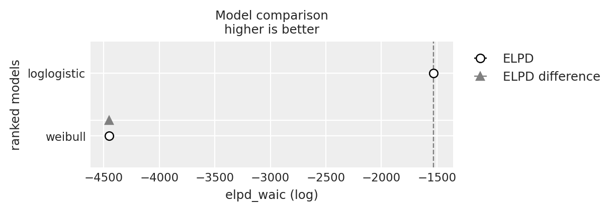
compare = az.compare({"weibull": weibull_idata, "loglogistic": loglogistic_idata}, ic="waic")
compare

	rank	elpd_waic	p_waic	elpd_diff	weight	se	dse	warning	scale
loglogistic	0	-1529.708134	12.302538	0.000000	1.0	28.919768	0.000000	False	log
weibull	1	-4449.052088	7.357847	2919.343954	0.0	14.245419	20.929315	False	log

az.plot_compare(compare);

从AFT模型推导个体生存预测

从上面我们可以看到回归方程是如何计算的，并作为\(\beta\)项进入Weibull似然函数，以及作为\(\mu\)参数进入逻辑分布。在这两种情况下，\(s\)参数仍然可以自由确定分布的形状。回想一下，回归方程在生存函数中作为时间点序列\(t\)的分母进入。

\[ S_{i}(t) = S_{0}\Bigg(\frac{t}{exp(\alpha_{i}x_{i} + \alpha_{2}x_{2} ... \alpha_{p}x_{p})}\Bigg) \]

因此，加权和越小，个体风险状况引起的加速因子就越大。

威布尔

每个个体案例的估计参数可以直接输入到Weibull生存函数中作为\(\beta\)项，以恢复预测的轨迹。

fig, axs = plt.subplots(1, 2, figsize=(20, 7))
axs = axs.flatten()
#### Using the fact that we've already stored expected value for the regression equation
reg = az.summary(weibull_idata, var_names=["reg"])["mean"]
t = np.arange(1, 13, 1)
s = az.summary(weibull_idata, var_names=["s"])["mean"][0]
axs[0].hist(reg, bins=30, ec="black", color="slateblue")
axs[0].set_title(
    "Histogram of Acceleration Factors in the individual Weibull fits \n across our sample"
)
axs[1].plot(
    t,
    weibull_min.sf(t, s, scale=reg.iloc[0]),
    label=r"Individual 1 - $\beta$: " + f"{reg.iloc[0]}," + r"$\alpha$: " + f"{s}",
)
axs[1].plot(
    t,
    weibull_min.sf(t, s, scale=reg.iloc[1000]),
    label=r"Individual 1000 - $\beta$: " + f"{reg.iloc[1000]}," + r"$\alpha$: " + f"{s}",
)
axs[1].set_title("Comparing Impact of Individual Factor \n on Survival Function")
axs[1].legend();

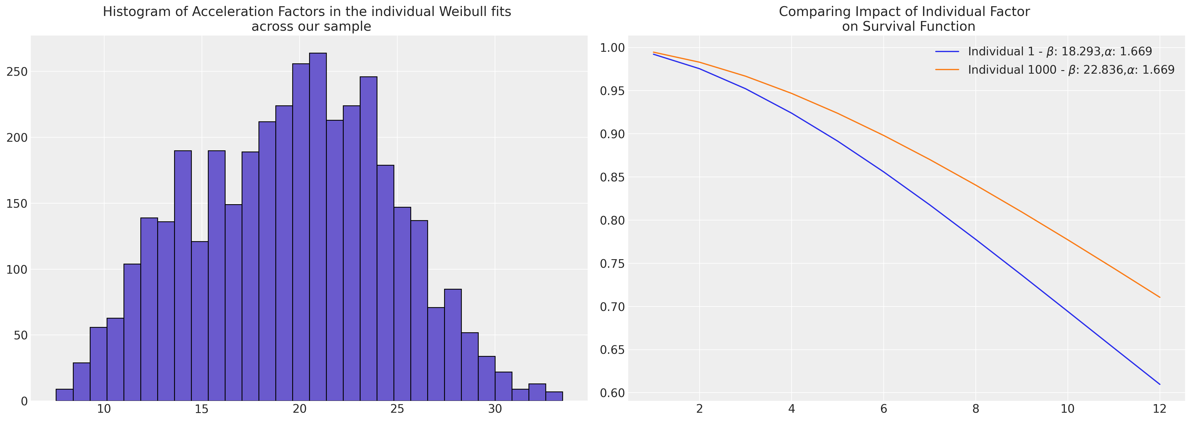
diff = reg.iloc[1000] - reg.iloc[0]
pchange = np.round(100 * (diff / reg.iloc[1000]), 2)
print(
    f"In this case we could think of the relative change in acceleration \n factor between the individuals as representing a {pchange}% increase"
)

In this case we could think of the relative change in acceleration 
 factor between the individuals as representing a 19.89% increase

reg = az.summary(weibull_idata, var_names=["reg"])["mean"]
s = az.summary(weibull_idata, var_names=["s"])["mean"][0]
t = np.arange(1, 13, 1)
weibull_predicted_surv = pd.DataFrame(
    [weibull_min.sf(t, s, scale=reg.iloc[i]) for i in range(len(reg))]
).T

weibull_predicted_surv

	0	1	2	3	4	5	6	7	8	9	...	3760	3761	3762	3763	3764	3765	3766	3767	3768	3769
0	0.992210	0.995004	0.989394	0.996205	0.985931	0.986630	0.993607	0.991524	0.984801	0.988076	...	0.992000	0.992905	0.977054	0.994145	0.994967	0.992228	0.995732	0.992615	0.992552	0.994143
1	0.975437	0.984199	0.966660	0.987982	0.955944	0.958101	0.979811	0.973296	0.952463	0.962572	...	0.974782	0.977613	0.928841	0.981499	0.984083	0.975495	0.986491	0.976704	0.976508	0.981495
2	0.952249	0.969150	0.935465	0.976494	0.915172	0.919238	0.960668	0.948141	0.908627	0.927698	...	0.950991	0.956432	0.864823	0.963927	0.968926	0.952360	0.973597	0.954684	0.954306	0.963919
3	0.923963	0.950613	0.897784	0.962283	0.866516	0.872748	0.937201	0.917528	0.856522	0.885767	...	0.921990	0.930531	0.790779	0.942347	0.950258	0.924136	0.957673	0.927784	0.927191	0.942334
4	0.891571	0.929133	0.855147	0.945732	0.812266	0.820757	0.910170	0.882575	0.798705	0.838585	...	0.888810	0.900784	0.711300	0.917431	0.928629	0.891814	0.939163	0.896928	0.896095	0.917413
5	0.855910	0.905157	0.808853	0.927149	0.754364	0.765074	0.880204	0.844222	0.737341	0.787690	...	0.852318	0.867922	0.630133	0.889738	0.904492	0.856226	0.918430	0.862888	0.861802	0.889714
6	0.817716	0.879077	0.760043	0.906799	0.694484	0.707264	0.847860	0.803302	0.674283	0.734421	...	0.813280	0.832589	0.550282	0.859756	0.878241	0.818106	0.895785	0.826349	0.825004	0.859726
7	0.777649	0.851242	0.709724	0.884919	0.634065	0.648678	0.813636	0.760557	0.611100	0.679952	...	0.772381	0.795365	0.474048	0.827927	0.850231	0.778112	0.871508	0.787922	0.786320	0.827891
8	0.736306	0.821975	0.658781	0.861727	0.574315	0.590467	0.777988	0.716655	0.549097	0.625299	...	0.730239	0.756774	0.403088	0.794653	0.820786	0.736840	0.845856	0.748163	0.746311	0.794610
9	0.694224	0.791570	0.607985	0.837421	0.516233	0.533589	0.741330	0.672191	0.489322	0.571326	...	0.687409	0.717293	0.338483	0.760301	0.790206	0.694824	0.819065	0.707573	0.705486	0.760253
10	0.651884	0.760303	0.557996	0.812190	0.460610	0.478819	0.704042	0.627695	0.432587	0.518759	...	0.644388	0.677354	0.280813	0.725212	0.758767	0.652545	0.791357	0.666605	0.664300	0.725158
11	0.609713	0.728426	0.509367	0.786208	0.408051	0.426760	0.666467	0.583629	0.379484	0.468183	...	0.601614	0.637342	0.230254	0.689694	0.726725	0.610428	0.762937	0.625662	0.623161	0.689635

12 行 × 3770 列

对数逻辑回归

在Logistic拟合的情况下，我们已经得到了需要转换的参数估计值，以恢复我们旨在估计的对数逻辑生存曲线。

reg = az.summary(loglogistic_idata, var_names=["reg"])["mean"]
s = az.summary(loglogistic_idata, var_names=["s"])["mean"][0]
temp = retention_df
t = np.log(np.arange(1, 13, 1))
## Transforming to the Log-Logistic scale
alpha = np.round((1 / s), 3)
beta = np.round(np.exp(reg) ** s, 3)

fig, axs = plt.subplots(1, 2, figsize=(20, 7))
axs = axs.flatten()
axs[0].hist(reg, bins=30, ec="black", color="slateblue")
axs[0].set_title("Histogram of beta terms in the individual Log Logistic fits")
axs[1].plot(
    np.exp(t),
    fisk.sf(t, c=alpha, scale=beta.iloc[0]),
    label=r"$\beta$: " + f"{beta.iloc[0]}," + r"$\alpha$: " + f"{alpha}",
)
axs[1].plot(
    np.exp(t),
    fisk.sf(t, c=alpha, scale=beta.iloc[1000]),
    label=r"$\beta$: " + f"{beta.iloc[1000]}," + r"$\alpha$: " + f"{alpha}",
)
axs[1].set_title("Comparing Impact of Individual Factor \n on Survival Function")
axs[1].legend();

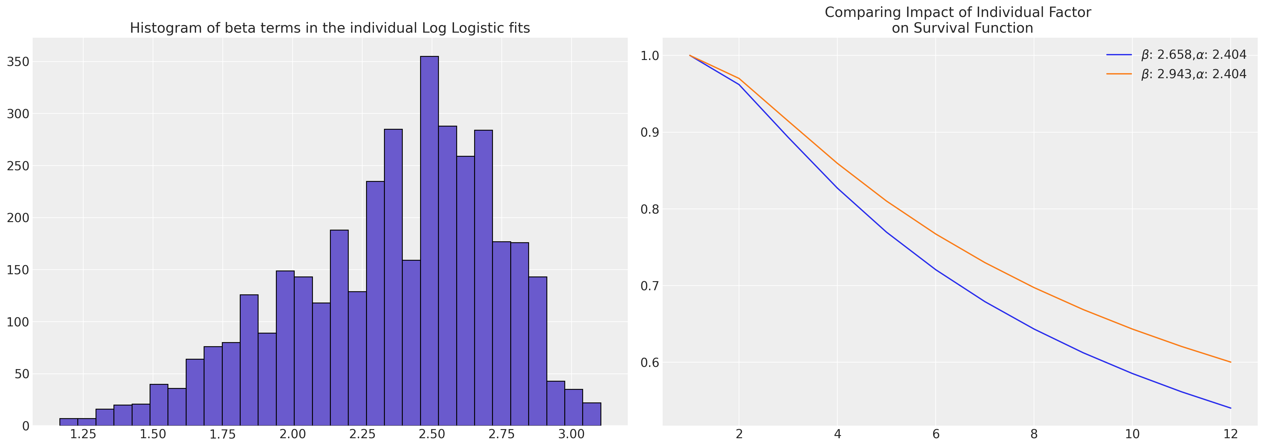
diff = beta.iloc[1000] - beta.iloc[0]
pchange = np.round(100 * (diff / beta.iloc[1000]), 2)
print(
    f"In this case we could think of the relative change in acceleration \n factor between the individuals as representing a {pchange}% increase"
)

In this case we could think of the relative change in acceleration 
 factor between the individuals as representing a 9.68% increase

loglogistic_predicted_surv = pd.DataFrame(
    [fisk.sf(t, c=alpha, scale=beta.iloc[i]) for i in range(len(reg))]
).T
loglogistic_predicted_surv

	0	1	2	3	4	5	6	7	8	9	...	3760	3761	3762	3763	3764	3765	3766	3767	3768	3769
0	1.000000	1.000000	1.000000	1.000000	1.000000	1.000000	1.000000	1.000000	1.000000	1.000000	...	1.000000	1.000000	1.000000	1.000000	1.000000	1.000000	1.000000	1.000000	1.000000	1.000000
1	0.961991	0.972250	0.950902	0.977471	0.939736	0.940788	0.967457	0.958955	0.936014	0.939485	...	0.959430	0.961925	0.916039	0.968951	0.969927	0.960809	0.975477	0.956383	0.961825	0.968190
2	0.893214	0.920502	0.864877	0.934806	0.837491	0.840024	0.907619	0.885339	0.828605	0.836887	...	0.886564	0.893041	0.782878	0.911612	0.914229	0.890136	0.929309	0.878736	0.892781	0.909577
3	0.827049	0.868761	0.785373	0.891275	0.746596	0.750123	0.848870	0.815305	0.734317	0.745757	...	0.817124	0.826790	0.673351	0.854996	0.859031	0.822444	0.882569	0.805554	0.826401	0.851869
4	0.769601	0.822189	0.718789	0.851325	0.672990	0.677099	0.796890	0.755111	0.658774	0.672014	...	0.757346	0.769280	0.590149	0.804638	0.809763	0.763902	0.839995	0.743183	0.768798	0.800678
5	0.720729	0.781302	0.663846	0.815635	0.613905	0.618336	0.751941	0.704345	0.598653	0.612855	...	0.706864	0.720364	0.526625	0.760888	0.766828	0.714270	0.802217	0.690957	0.719817	0.756311
6	0.679108	0.745520	0.618238	0.783917	0.565951	0.570547	0.713119	0.661429	0.550193	0.564863	...	0.664139	0.678713	0.477065	0.722952	0.729499	0.672124	0.768845	0.647072	0.678120	0.717917
7	0.643393	0.714085	0.579939	0.755671	0.526425	0.531093	0.679403	0.624834	0.510473	0.525321	...	0.627672	0.642978	0.437489	0.689888	0.696890	0.636049	0.739284	0.609840	0.642354	0.684515
8	0.612462	0.686296	0.547375	0.730397	0.493338	0.498021	0.649896	0.593311	0.477377	0.492230	...	0.596233	0.612032	0.405209	0.660864	0.668205	0.604872	0.712959	0.577908	0.611387	0.655239
9	0.585422	0.661562	0.519359	0.707659	0.465244	0.469908	0.623864	0.565882	0.449386	0.464142	...	0.568859	0.584983	0.378386	0.635191	0.642787	0.577668	0.689376	0.550228	0.584323	0.629379
10	0.561578	0.639400	0.494993	0.687088	0.441087	0.445710	0.600723	0.541794	0.425398	0.439995	...	0.544803	0.561133	0.355739	0.612313	0.620101	0.553718	0.668121	0.525999	0.560464	0.606363
11	0.540383	0.619416	0.473595	0.668376	0.420081	0.424652	0.580005	0.520459	0.404598	0.419003	...	0.523484	0.539933	0.336352	0.591787	0.599718	0.532459	0.648855	0.504600	0.539258	0.585735

12 行 × 3770 列

这两个模型对这两个个体的拟合估计值相当。我们现在将看到边际生存函数在整个个体样本中的比较情况。

fig, ax = plt.subplots(figsize=(20, 7))
ax.plot(
    loglogistic_predicted_surv.iloc[:, [1, 300]], label=["LL-Individual 1", "LL-Individual 300"]
)
ax.plot(
    loglogistic_predicted_surv.mean(axis=1),
    label="LL Marginal Survival Curve",
    linestyle="--",
    color="black",
    linewidth=4.5,
)
ax.plot(weibull_predicted_surv.iloc[:, [1, 300]], label=["W-Individual 1", "W-Individual 300"])
ax.plot(
    weibull_predicted_surv.mean(axis=1),
    label="W Marginal Survival Curve",
    linestyle="dotted",
    color="black",
    linewidth=4.5,
)
ax.plot(surv_df.iloc[:, [1, 300]], label=["CoxPH-Individual 1", "CoxPH-Individual 300"])
ax.plot(
    surv_df.mean(axis=1),
    label="CoxPH Marginal Survival Curve",
    linestyle="-.",
    color="black",
    linewidth=4.5,
)
ax.set_title(
    "Comparison predicted Individual Survival Curves and \n Marginal (expected) Survival curve across Sample",
    fontsize=25,
)
kmf.plot_survival_function(ax=ax, label="Overall KM estimate", color="black")
ax.set_xlabel("Time in Month")
ax.set_ylabel("Probability")
ax.legend();

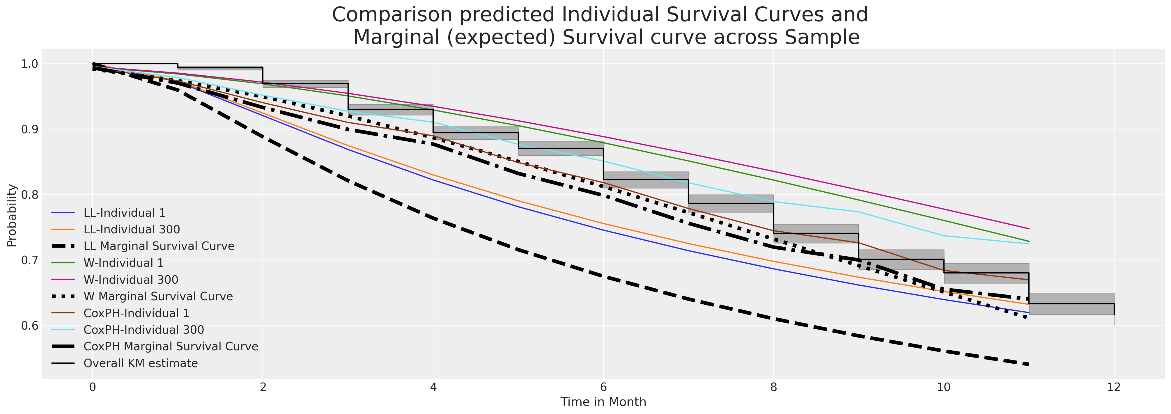
上面我们绘制了每个模型中个体预测生存函数的样本。此外，我们还绘制了通过在我们的数据集中对个体样本进行行平均预测的边际生存曲线。这个边际量通常是用于比较不同时间段变化的实用基准。它是一个可以逐年和随时比较的指标。

通过个体拟合具有共享脆弱项的模型

在贝叶斯回归建模中，最具吸引力的模式之一是能够结合层次结构。层次生存模型的类似物是个体脆弱性生存模型。但“脆弱性”不必仅在个体层面指定——所谓的“共享”脆弱性可以在组层面部署，例如在field范围内。

在上面的CoxPH模型中，我们将数据拟合到一个标准的回归公式中，使用指示变量来表示field变量的不同水平，这些变量被包含在加权线性组合的总和中。在脆弱性模型中，我们允许个体或群体脆弱性项作为乘法因子进入我们的模型，除了基线危险与加权人口特征的组合之外。这使我们能够捕捉到作为特定个体或特定群体的异质效应的估计。在我们的情境中，这些项试图解释一些员工尽管市场上有其他机会，但仍对公司表现出“过度”的长期忠诚度。此外，我们可以对基线危险进行分层，例如按性别，以捕捉随着时间的推移，作为其协变量配置文件的函数，风险的不同程度。因此，我们的方程现在变为：

\[ \lambda_{i}(t) = z_{i}exp(\beta X)\lambda_{0}^{g}(t) \]

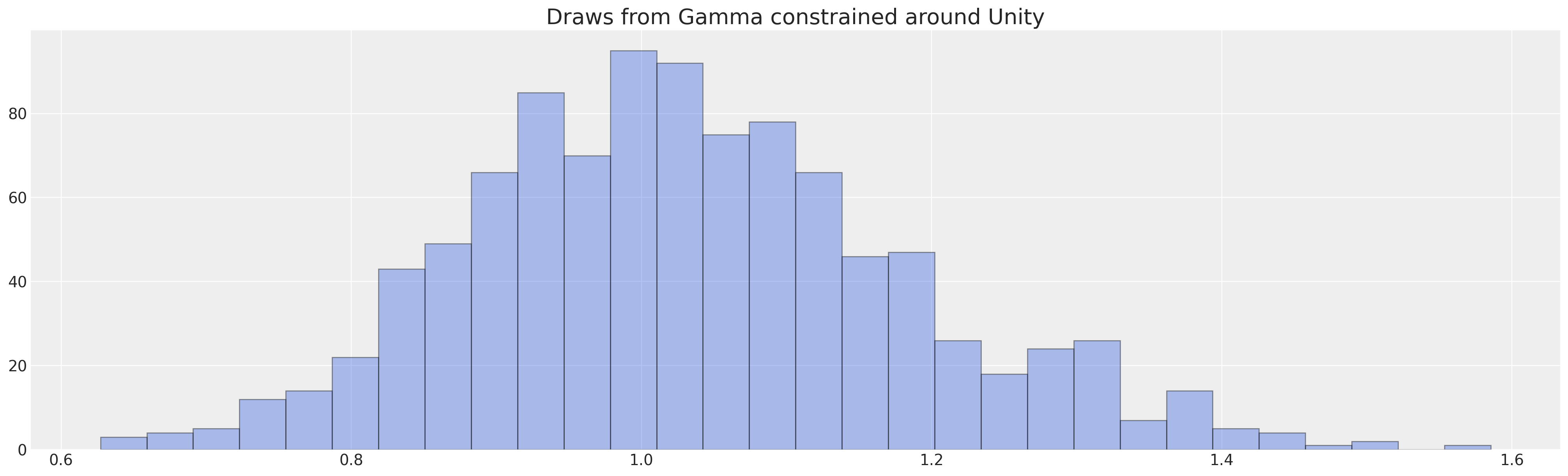
这可以通过贝叶斯方式进行估计，如下所示。注意我们必须对乘法进入方程的\(z\)项设置先验。为了设置这样的先验，我们推理个体异质性不会导致时间到流失的速度加快/减慢超过30%，并且我们选择伽马分布作为我们脆弱项的先验。

opt_params = pm.find_constrained_prior(
    pm.Gamma,
    lower=0.80,
    upper=1.30,
    mass=0.90,
    init_guess={"alpha": 1.7, "beta": 1.7},
)

opt_params

/Users/nathanielforde/mambaforge/envs/pymc_examples_new/lib/python3.9/site-packages/pytensor/tensor/rewriting/elemwise.py:685: UserWarning: Optimization Warning: The Op gammainc_der does not provide a C implementation. As well as being potentially slow, this also disables loop fusion.
  warn(
/Users/nathanielforde/mambaforge/envs/pymc_examples_new/lib/python3.9/site-packages/pytensor/tensor/rewriting/elemwise.py:685: UserWarning: Optimization Warning: The Op gammainc_der does not provide a C implementation. As well as being potentially slow, this also disables loop fusion.
  warn(

{'alpha': 46.22819238464343, 'beta': 44.910852755302585}

fig, ax = plt.subplots(figsize=(20, 6))
ax.hist(
    pm.draw(pm.Gamma.dist(alpha=opt_params["alpha"], beta=opt_params["beta"]), 1000),
    ec="black",
    color="royalblue",
    bins=30,
    alpha=0.4,
)
ax.set_title("Draws from Gamma constrained around Unity", fontsize=20);

preds = [
    "sentiment",
    "intention",
    "Low",
    "Medium",
    "Finance",
    "Health",
    "Law",
    "Public/Government",
    "Sales/Marketing",
]
preds3 = ["sentiment", "Low", "Medium"]


def make_coxph_frailty(preds, factor):
    frailty_idx, frailty_labels = pd.factorize(factor)
    df_m = retention_df[retention_df["Male"] == 1]
    df_f = retention_df[retention_df["Male"] == 0]
    coords = {
        "intervals": intervals,
        "preds": preds,
        "frailty_id": frailty_labels,
        "gender": ["Male", "Female"],
        "women": df_f.index,
        "men": df_m.index,
        "obs": range(len(retention_df)),
    }

    with pm.Model(coords=coords) as frailty_model:
        X_data_m = pm.MutableData("X_data_m", df_m[preds], dims=("men", "preds"))
        X_data_f = pm.MutableData("X_data_f", df_f[preds], dims=("women", "preds"))
        lambda0 = pm.Gamma("lambda0", 0.01, 0.01, dims=("intervals", "gender"))
        sigma_frailty = pm.Normal("sigma_frailty", opt_params["alpha"], 1)
        mu_frailty = pm.Normal("mu_frailty", opt_params["beta"], 1)
        frailty = pm.Gamma("frailty", mu_frailty, sigma_frailty, dims="frailty_id")

        beta = pm.Normal("beta", 0, sigma=1, dims="preds")

        ## Stratified baseline hazards
        lambda_m = pm.Deterministic(
            "lambda_m",
            pt.outer(pt.exp(pm.math.dot(beta, X_data_m.T)), lambda0[:, 0]),
            dims=("men", "intervals"),
        )
        lambda_f = pm.Deterministic(
            "lambda_f",
            pt.outer(pt.exp(pm.math.dot(beta, X_data_f.T)), lambda0[:, 1]),
            dims=("women", "intervals"),
        )
        lambda_ = pm.Deterministic(
            "lambda_",
            frailty[frailty_idx, None] * pt.concatenate([lambda_f, lambda_m], axis=0),
            dims=("obs", "intervals"),
        )

        mu = pm.Deterministic("mu", exposure * lambda_, dims=("obs", "intervals"))

        obs = pm.Poisson("outcome", mu, observed=quit, dims=("obs", "intervals"))
        frailty_idata = pm.sample(random_seed=101)

    return frailty_idata, frailty_model


frailty_idata, frailty_model = make_coxph_frailty(preds, range(len(retention_df)))
pm.model_to_graphviz(frailty_model)

Auto-assigning NUTS sampler...
Initializing NUTS using jitter+adapt_diag...
Multiprocess sampling (4 chains in 4 jobs)
NUTS: [lambda0, sigma_frailty, mu_frailty, frailty, beta]

100.00% [8000/8000 02:42<00:00 Sampling 4 chains, 0 divergences]

Sampling 4 chains for 1_000 tune and 1_000 draw iterations (4_000 + 4_000 draws total) took 162 seconds.
The rhat statistic is larger than 1.01 for some parameters. This indicates problems during sampling. See https://arxiv.org/abs/1903.08008 for details
The effective sample size per chain is smaller than 100 for some parameters.  A higher number is needed for reliable rhat and ess computation. See https://arxiv.org/abs/1903.08008 for details

拟合上述模型使我们能够提取出基于性别的基准风险视图。这种模型规范可以帮助解释比例风险假设的失败，允许表达由协变量不同水平引起的时间变化风险。我们还可以允许在组之间共享脆弱项，如在基于工作领域的组效应情况下。然而，这通常与在第一个CoxPH模型中将领域作为固定效应包括在内没有太大区别，但在这里我们允许系数估计值来自相同的分布。该分布的方差特性可能具有独立兴趣。

这里的方差越大，基础模型在捕捉观察到的状态转换方面就越差。在思考索里托斯悖论背景下的演变风险时，你可能会认为个体脆弱性项的异质性越大，模型越不明确，我们对所讨论状态转换的理解就越差，从而导致沙子何时成为堆的语义模糊性，以及员工何时可能离职的不确定性增加。

接下来，我们将在field分组中拟合一个包含脆弱性的模型。这些被称为共享脆弱性。

shared_frailty_idata, shared_frailty_model = make_coxph_frailty(preds3, retention_df["field"])

Auto-assigning NUTS sampler...
Initializing NUTS using jitter+adapt_diag...
Multiprocess sampling (4 chains in 4 jobs)
NUTS: [lambda0, sigma_frailty, mu_frailty, frailty, beta]

100.00% [8000/8000 01:11<00:00 Sampling 4 chains, 0 divergences]

Sampling 4 chains for 1_000 tune and 1_000 draw iterations (4_000 + 4_000 draws total) took 71 seconds.

pm.model_to_graphviz(shared_frailty_model)

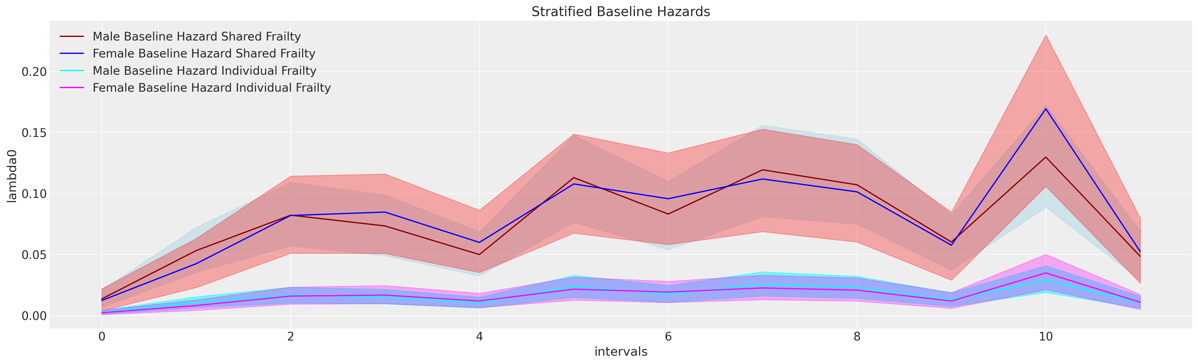
共享和个体脆弱项之间的比较使我们能够看到，包含更多的协变量和个体脆弱项如何吸收基准风险中的方差并缩小潜在风险的幅度。

fig, ax = plt.subplots(figsize=(20, 6))
base_m = shared_frailty_idata["posterior"]["lambda0"].sel(gender="Male")
base_f = shared_frailty_idata["posterior"]["lambda0"].sel(gender="Female")
az.plot_hdi(range(12), base_m, ax=ax, color="lightblue", fill_kwargs={"alpha": 0.5}, smooth=False)
az.plot_hdi(range(12), base_f, ax=ax, color="red", fill_kwargs={"alpha": 0.3}, smooth=False)
get_mean(base_m).plot(ax=ax, color="darkred", label="Male Baseline Hazard Shared Frailty")
get_mean(base_f).plot(ax=ax, color="blue", label="Female Baseline Hazard Shared Frailty")

base_m_i = frailty_idata["posterior"]["lambda0"].sel(gender="Male")
base_f_i = frailty_idata["posterior"]["lambda0"].sel(gender="Female")
az.plot_hdi(range(12), base_m_i, ax=ax, color="cyan", fill_kwargs={"alpha": 0.5}, smooth=False)
az.plot_hdi(range(12), base_f_i, ax=ax, color="magenta", fill_kwargs={"alpha": 0.3}, smooth=False)
get_mean(base_m_i).plot(ax=ax, color="cyan", label="Male Baseline Hazard Individual Frailty")
get_mean(base_f_i).plot(ax=ax, color="magenta", label="Female Baseline Hazard Individual Frailty")


ax.legend()
ax.set_title("Stratified Baseline Hazards");

让我们提取并检查各个脆弱性项：

frailty_terms = az.summary(frailty_idata, var_names=["frailty"])
frailty_terms.head()

	mean	sd	hdi_3%	hdi_97%	mcse_mean	mcse_sd	ess_bulk	ess_tail	r_hat
frailty[0]	0.959	0.146	0.678	1.223	0.003	0.002	2433.0	2325.0	1.0
frailty[1]	0.984	0.152	0.692	1.255	0.003	0.002	2352.0	2273.0	1.0
frailty[2]	0.980	0.145	0.699	1.243	0.003	0.002	3027.0	2771.0	1.0
frailty[3]	0.963	0.143	0.705	1.247	0.003	0.002	2174.0	2785.0	1.0
frailty[4]	0.953	0.141	0.687	1.217	0.004	0.003	1508.0	2561.0	1.0

以及各组之间的共享术语。我们可以看到，在控制其他人口统计信息后，无论是在财务还是健康领域工作，似乎都会增加离职的可能性。

axs = az.plot_posterior(shared_frailty_idata, var_names=["frailty"])
axs = axs.flatten()
for ax in axs:
    ax.axvline(1, color="red", label="No change")
    ax.legend()
plt.suptitle("Shared Frailty Estimates across the Job Area", fontsize=30);

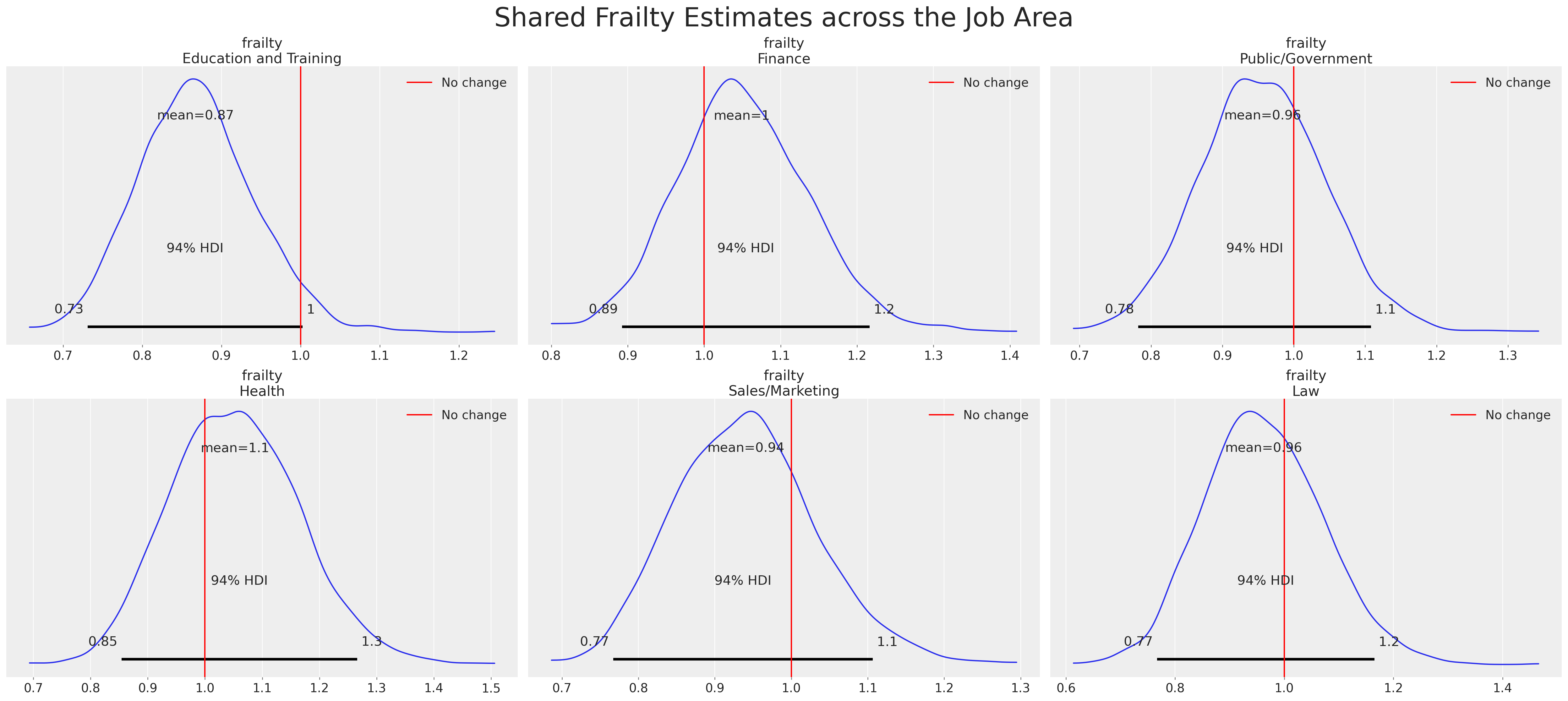
共享脆弱性模型（如本例中的模型）在某些情况下非常重要，例如在医学试验中，我们希望测量实施试验协议的机构之间的差异。同样，在人力资源背景下，我们可能会考虑研究不同管理者/团队动态下的差异脆弱性项。

目前我们将暂时搁置这一建议，专注于个体脆弱性模型。

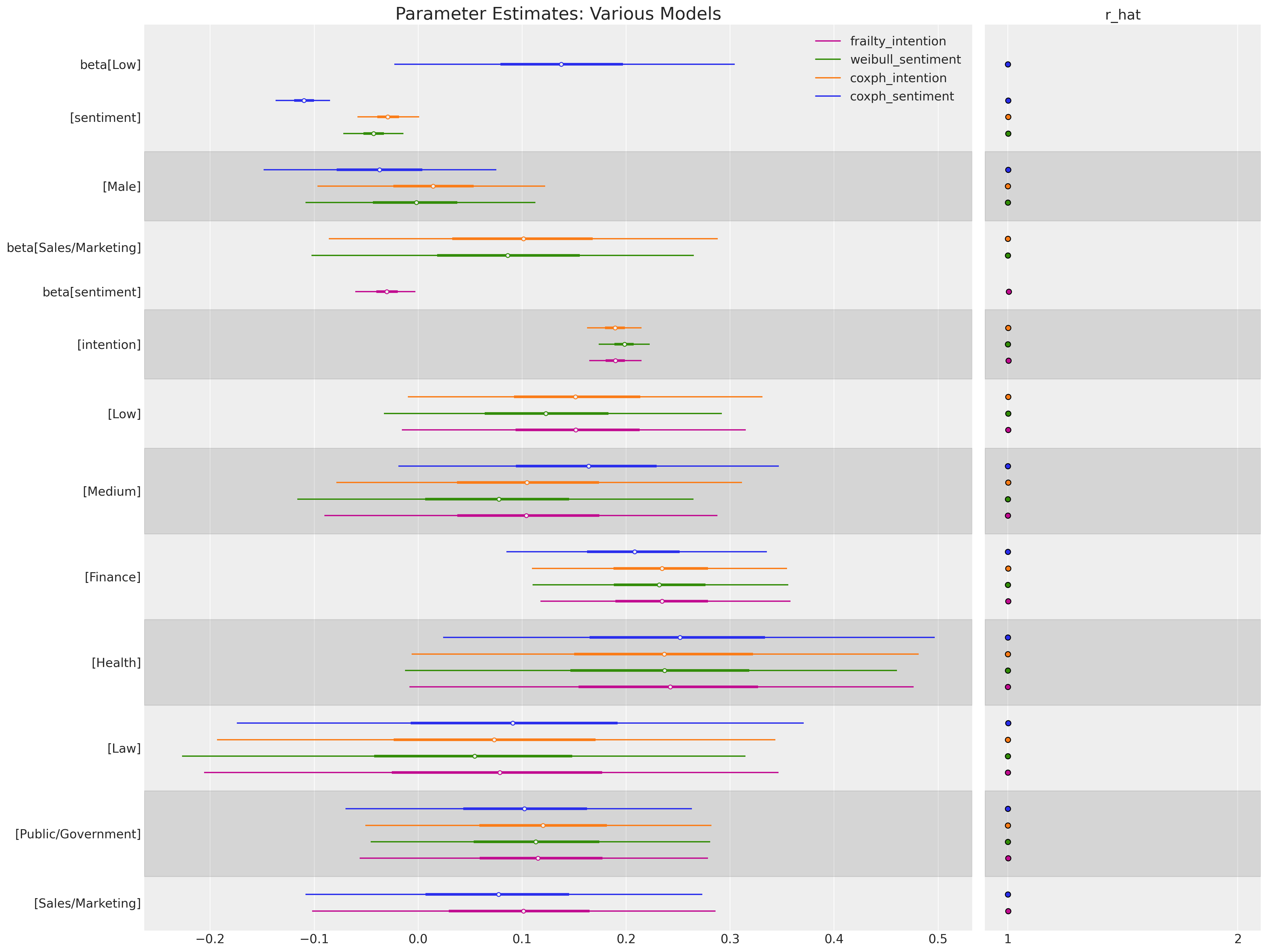
ax = az.plot_forest(
    [base_idata, base_intention_idata, weibull_idata, frailty_idata],
    model_names=["coxph_sentiment", "coxph_intention", "weibull_sentiment", "frailty_intention"],
    var_names=["beta"],
    combined=True,
    figsize=(20, 15),
    r_hat=True,
)

ax[0].set_title("Parameter Estimates: Various Models", fontsize=20);

我们现在可以将脆弱性估计值分解，并将其与我们已知的每个个体的 demographic 信息进行比较。由于我们在建模时没有使用 intention 变量，因此看到模型如何尝试通过个体脆弱性项来补偿 stated intention 的影响是很有趣的。

temp = retention_df.copy()
temp["frailty"] = frailty_terms.reset_index()["mean"]
(
    temp.groupby(["Male", "sentiment", "intention"])[["frailty"]]
    .mean()
    .reset_index()
    .pivot(index=["Male", "sentiment"], columns="intention", values="frailty")
    .style.background_gradient(cmap="OrRd", axis=None)
    .set_precision(3)
)

/var/folders/__/ng_3_9pn1f11ftyml_qr69vh0000gn/T/ipykernel_48265/2005202898.py:4: FutureWarning: this method is deprecated in favour of `Styler.format(precision=..)`
  temp.groupby(["Male", "sentiment", "intention"])[["frailty"]]

	intention	1	2	3	4	5	6	7	8	9	10
Male	sentiment
0	1	nan	0.983	nan	nan	nan	0.981	nan	0.986	0.961	0.982
	2	0.966	nan	nan	0.970	0.973	0.963	0.963	0.972	0.986	0.962
	3	0.989	0.975	0.971	0.972	0.970	0.964	0.965	0.974	nan	0.995
	4	0.972	0.971	0.985	0.970	0.975	0.968	0.970	0.965	0.973	nan
	5	nan	0.961	0.986	0.978	0.964	0.963	0.974	0.964	nan	0.947
	6	0.976	0.970	0.961	0.965	0.978	0.966	0.960	0.978	nan	0.986
	7	0.972	0.969	0.969	0.973	0.969	0.972	0.969	0.969	0.968	0.965
	8	0.968	0.969	0.969	0.969	0.968	0.971	0.968	0.968	0.968	0.958
	9	0.970	0.970	0.969	0.967	0.966	0.971	0.969	0.950	nan	nan
	10	0.967	0.971	0.968	0.971	0.970	0.970	0.974	0.953	0.960	nan
1	1	nan	nan	0.975	nan	0.968	0.981	0.951	0.969	0.965	0.975
	2	nan	0.973	0.972	0.967	0.964	0.972	0.966	0.965	0.970	0.983
	3	0.962	nan	0.989	0.967	0.965	0.969	0.955	0.968	0.960	0.981
	4	nan	0.971	0.966	0.973	0.971	0.971	0.970	0.976	0.969	nan
	5	0.965	0.976	0.967	0.966	0.981	0.974	0.963	0.974	0.947	0.946
	6	0.972	0.968	0.964	0.969	0.970	0.961	0.968	0.964	0.979	0.972
	7	0.967	0.971	0.969	0.969	0.968	0.971	0.971	0.965	0.970	0.975
	8	0.969	0.970	0.968	0.969	0.970	0.972	0.971	0.973	0.976	0.978
	9	0.970	0.970	0.968	0.969	0.970	0.964	0.964	0.973	0.974	nan
	10	0.968	0.970	0.969	0.972	0.969	0.967	0.970	0.977	0.988	nan

上述热图表明，模型特别过度权衡了低情感和低意图得分的影响。脆弱项通过增加危害项乘法增加率的减少来补偿。总体上，模型过度权衡了风险，这种风险被脆弱项向下“修正”。这在某种程度上是有道理的，因为看到如此低的情感与没有离职意图相结合是有点奇怪的。这表明受访者的回答可能没有反映他们的深思熟虑的意见。在离职意图较高的情况下，这种效果同样明显，这在当前背景下也是有道理的。

询问Cox脆弱模型

与之前一样，我们希望提取出单独的预测生存函数和累积风险函数。这可以类似于上述分析来完成，但在这里我们包含了平均脆弱项来预测个体风险。

def extract_individual_frailty(i, retention_df, intention=False):
    beta = frailty_idata.posterior["beta"]
    if intention:
        intention_posterior = beta.sel(preds="intention")
    else:
        intention_posterior = 0
    hazard_base_m = frailty_idata["posterior"]["lambda0"].sel(gender="Male")
    hazard_base_f = frailty_idata["posterior"]["lambda0"].sel(gender="Female")
    frailty = frailty_idata.posterior["frailty"]
    if retention_df.iloc[i]["Male"] == 1:
        hazard_base = hazard_base_m
    else:
        hazard_base = hazard_base_f

    full_hazard_idata = hazard_base * (
        frailty.sel(frailty_id=i).mean().item()
        * np.exp(
            beta.sel(preds="sentiment") * retention_df.iloc[i]["sentiment"]
            + np.where(intention, intention_posterior * retention_df.iloc[i]["intention"], 0)
            + beta.sel(preds="Low") * retention_df.iloc[i]["Low"]
            + beta.sel(preds="Medium") * retention_df.iloc[i]["Medium"]
            + beta.sel(preds="Finance") * retention_df.iloc[i]["Finance"]
            + beta.sel(preds="Health") * retention_df.iloc[i]["Health"]
            + beta.sel(preds="Law") * retention_df.iloc[i]["Law"]
            + beta.sel(preds="Public/Government") * retention_df.iloc[i]["Public/Government"]
            + beta.sel(preds="Sales/Marketing") * retention_df.iloc[i]["Sales/Marketing"]
        )
    )

    cum_haz_idata = cum_hazard(full_hazard_idata)
    survival_idata = survival(full_hazard_idata)
    return full_hazard_idata, cum_haz_idata, survival_idata, hazard_base


def plot_individual_frailty(retention_df, individuals=[1, 300, 700], intention=False):
    fig, axs = plt.subplots(1, 2, figsize=(20, 7))
    axs = axs.flatten()
    colors = ["slateblue", "magenta", "darkgreen"]
    for i, c in zip(individuals, colors):
        haz_idata, cum_haz_idata, survival_idata, base_hazard = extract_individual_frailty(
            i, retention_df, intention
        )
        axs[0].plot(get_mean(survival_idata), label=f"individual_{i}", color=c)
        az.plot_hdi(range(12), survival_idata, ax=axs[0], fill_kwargs={"color": c})
        axs[1].plot(get_mean(cum_haz_idata), label=f"individual_{i}", color=c)
        az.plot_hdi(range(12), cum_haz_idata, ax=axs[1], fill_kwargs={"color": c})
        axs[0].set_title("Individual Survival Functions", fontsize=20)
        axs[1].set_title("Individual Cumulative Hazard Functions", fontsize=20)
    az.plot_hdi(
        range(12),
        survival(base_hazard),
        color="lightblue",
        ax=axs[0],
        fill_kwargs={"label": "Baseline Survival"},
    )
    az.plot_hdi(
        range(12),
        cum_hazard(base_hazard),
        color="lightblue",
        ax=axs[1],
        fill_kwargs={"label": "Baseline Hazard"},
    )
    axs[0].legend()
    axs[1].legend()


plot_individual_frailty(retention_df, [0, 1, 2], intention=True)

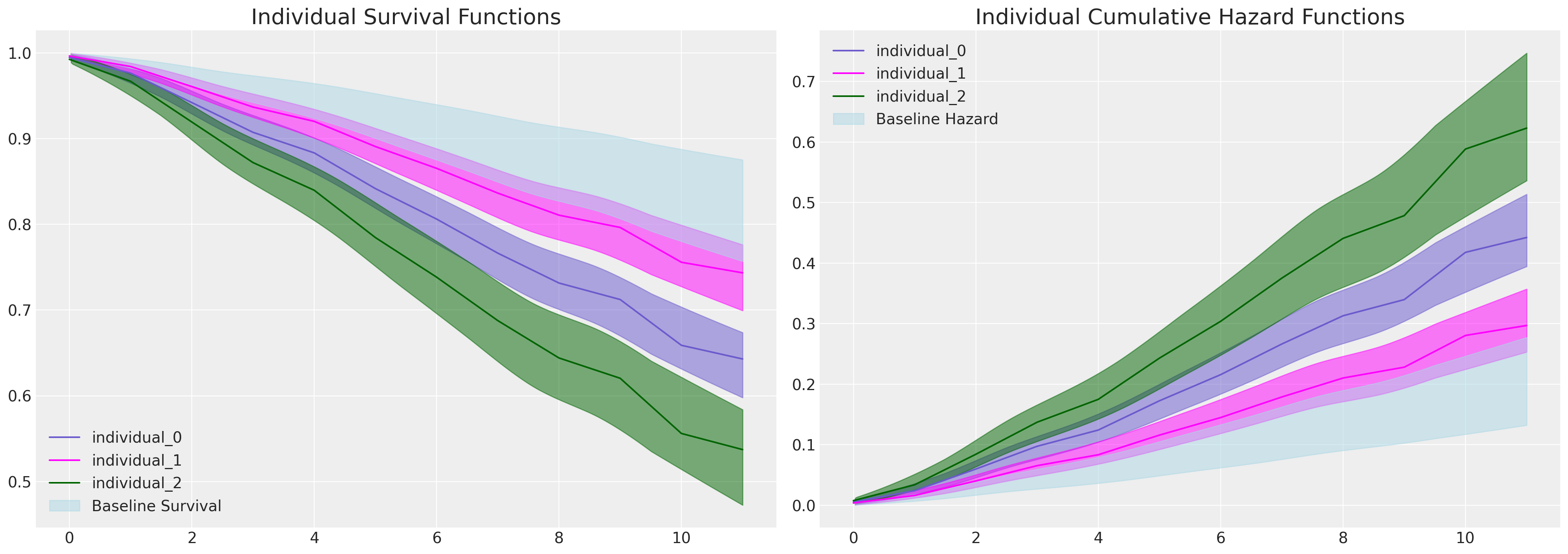
在这些图中，我们看到每个个体预测的生存函数之间存在显著差异，这种差异可以通过他们表达的离职意图来解释。通过检查这三个个体的协变量特征，我们可以看到这一点。

retention_df.iloc[0:3, :]

	gender	field	level	sentiment	intention	left	month	Male	Low	Medium	Finance	Health	Law	Public/Government	Sales/Marketing
0	F	Education and Training	Low	8	5	0	12	0	1	0	0	0	0	0	0
1	F	Education and Training	Medium	8	3	1	11	0	0	1	0	0	0	0	0
2	F	Education and Training	Low	10	7	1	9	0	1	0	0	0	0	0	0

def create_predictions(retention_df, intention=False):
    cum_haz = {}
    surv = {}
    for i in range(len(retention_df)):
        haz_idata, cum_haz_idata, survival_idata, base_hazard = extract_individual_frailty(
            i, retention_df, intention
        )
        cum_haz[i] = get_mean(cum_haz_idata)
        surv[i] = get_mean(survival_idata)
    cum_haz = pd.DataFrame(cum_haz)
    surv = pd.DataFrame(surv)
    return cum_haz, surv


cum_haz_frailty_df, surv_frailty_df = create_predictions(retention_df, intention=True)
surv_frailty_df

	0	1	2	3	4	5	6	7	8	9	...	3760	3761	3762	3763	3764	3765	3766	3767	3768	3769
0	0.994606	0.996375	0.992411	0.997349	0.990543	0.990702	0.995489	0.994179	0.989593	0.991453	...	0.993628	0.994188	0.983980	0.995030	0.995925	0.993665	0.996433	0.994158	0.994063	0.995216
1	0.976327	0.984043	0.966826	0.988325	0.958788	0.959467	0.980174	0.974480	0.954712	0.962651	...	0.969320	0.971975	0.924277	0.976007	0.980310	0.969484	0.982735	0.971909	0.971377	0.976890
2	0.942033	0.960706	0.919347	0.971156	0.900424	0.902001	0.951311	0.937624	0.890904	0.909467	...	0.932821	0.938532	0.838909	0.947254	0.956586	0.933182	0.961883	0.938401	0.937252	0.949165
3	0.907312	0.936786	0.872011	0.953446	0.842969	0.845380	0.921911	0.900423	0.828493	0.856838	...	0.900804	0.909106	0.768149	0.921832	0.935513	0.901336	0.943293	0.908935	0.907248	0.924625
4	0.883317	0.920081	0.839730	0.941000	0.804224	0.807162	0.901485	0.874762	0.786641	0.821132	...	0.879373	0.889368	0.722899	0.904702	0.921262	0.880021	0.930687	0.889181	0.887128	0.908082
5	0.841648	0.890708	0.784532	0.918977	0.738834	0.742598	0.865795	0.830381	0.716478	0.760581	...	0.832603	0.846130	0.629919	0.866986	0.889720	0.833480	0.902695	0.845922	0.843086	0.871607
6	0.806120	0.865288	0.738349	0.899763	0.684982	0.689352	0.835135	0.792668	0.659146	0.710355	...	0.799519	0.815422	0.568818	0.840028	0.867017	0.800552	0.882474	0.815213	0.811833	0.845499
7	0.766357	0.836395	0.687650	0.877734	0.626822	0.631774	0.800555	0.750613	0.597743	0.655685	...	0.753924	0.772917	0.490788	0.802467	0.835171	0.755166	0.853987	0.772734	0.768621	0.809073
8	0.731486	0.810657	0.644064	0.857939	0.577659	0.583025	0.769986	0.713897	0.546274	0.609121	...	0.714991	0.736461	0.429643	0.769989	0.807437	0.716402	0.829057	0.736314	0.731583	0.777532
9	0.712245	0.796290	0.620376	0.846812	0.551281	0.556847	0.753018	0.693707	0.518844	0.584005	...	0.693743	0.716486	0.398343	0.752098	0.792068	0.695239	0.815195	0.716379	0.711309	0.760135
10	0.658844	0.755713	0.556014	0.815095	0.480884	0.486882	0.705519	0.637894	0.446305	0.516415	...	0.649420	0.674652	0.337641	0.714375	0.759462	0.651082	0.785667	0.674635	0.668877	0.723405
11	0.642894	0.743387	0.537195	0.805370	0.460674	0.466766	0.691211	0.621300	0.425672	0.496850	...	0.633592	0.659655	0.317438	0.700771	0.747627	0.635315	0.774906	0.659680	0.653684	0.710145

12 行 × 3770 列

cm_subsection = np.linspace(0, 1, 120)
colors_m = [cm.Purples(x) for x in cm_subsection]
colors = [cm.spring(x) for x in cm_subsection]


fig, axs = plt.subplots(1, 2, figsize=(20, 7))
axs = axs.flatten()
cum_haz_frailty_df.plot(legend=False, color=colors, alpha=0.05, ax=axs[1])
axs[1].plot(cum_haz_frailty_df.mean(axis=1), color="black", linewidth=4)
axs[1].set_title(
    "Predicted Individual Cumulative Hazard \n & Expected Cumulative Hazard", fontsize=20
)

surv_frailty_df.plot(legend=False, color=colors_m, alpha=0.05, ax=axs[0])
axs[0].plot(surv_frailty_df.mean(axis=1), color="black", linewidth=4)
axs[0].set_title("Predicted Individual Survival Curves \n  & Expected Survival Curve", fontsize=20)
axs[0].annotate(
    f"Expected Attrition by 6 months: {np.round(1-surv_frailty_df.mean(axis=1).iloc[6], 3)}",
    (2, 0.5),
    fontsize=12,
    fontweight="bold",
);

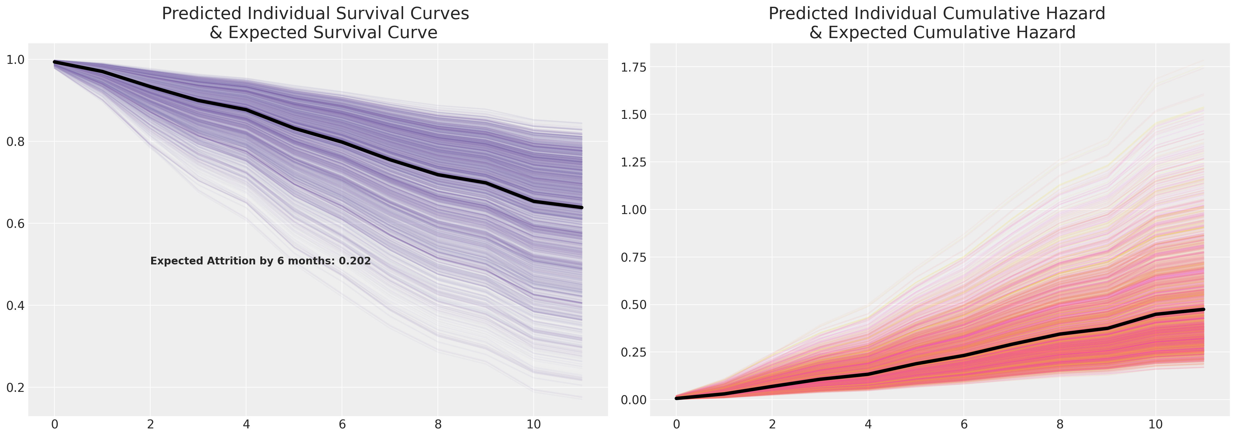
请注意，与上述Cox模型相比，我们的额外脆弱项导致的生存曲线范围增加。

绘制脆弱项的影响

有不同的方法可以对数据进行边缘化处理，但我们也可以检查个体的“脆弱性”。这类图表和调查在政策转变的背景下最为有效。你想确定那些亲身经历政策转变的人与那些没有经历政策转变的人之间的反应差异率。这有助于聚焦于受影响最大的员工或研究参与者，以找出是否有任何因素驱动了他们的反应，以及是否需要采取预防措施来解决危机。

beta_individual_all = frailty_idata["posterior"]["frailty"]
predicted_all = beta_individual_all.mean(("chain", "draw"))
predicted_all = predicted_all.sortby(predicted_all, ascending=False)
beta_individual = beta_individual_all.sel(frailty_id=range(500))
predicted = beta_individual.mean(("chain", "draw"))
predicted = predicted.sortby(predicted, ascending=False)
ci_lb = beta_individual.quantile(0.025, ("chain", "draw")).sortby(predicted)
ci_ub = beta_individual.quantile(0.975, ("chain", "draw")).sortby(predicted)
hdi = az.hdi(beta_individual, hdi_prob=0.5).sortby(predicted)
hdi2 = az.hdi(beta_individual, hdi_prob=0.8).sortby(predicted)

cm_subsection = np.linspace(0, 1, 500)
colors = [cm.cool(x) for x in cm_subsection]

fig = plt.figure(figsize=(20, 10))
gs = fig.add_gridspec(
    2,
    2,
    height_ratios=(1, 7),
    left=0.1,
    right=0.9,
    bottom=0.1,
    top=0.9,
    wspace=0.05,
    hspace=0.05,
)
# Create the Axes.
ax = fig.add_subplot(gs[1, 0])
ax.set_yticklabels([])
ax_histx = fig.add_subplot(gs[0, 0], sharex=ax)
ax_histx.set_title("Expected Frailty Terms per Individual Risk Profile", fontsize=20)
ax_histx.hist(predicted_all, bins=30, color="slateblue")
ax_histx.set_yticklabels([])
ax_histx.tick_params(labelsize=8)
ax.set_ylabel("Individual Frailty Terms", fontsize=18)
ax.tick_params(labelsize=8)
ax.hlines(
    range(len(predicted)),
    hdi.sel(hdi="lower").to_array(),
    hdi.sel(hdi="higher").to_array(),
    color=colors,
    label="50% HDI",
    linewidth=0.8,
)
ax.hlines(
    range(len(predicted)),
    hdi2.sel(hdi="lower").to_array(),
    hdi2.sel(hdi="higher").to_array(),
    color="green",
    alpha=0.2,
    label="80% HDI",
    linewidth=0.8,
)
ax.set_xlabel("Multiplicative Effect of Individual Frailty", fontsize=18)
ax.legend()
ax.fill_betweenx(range(len(predicted)), 0.95, 1.0, alpha=0.4, color="grey")

ax1 = fig.add_subplot(gs[1, 1])
f_index = retention_df[retention_df["gender"] == "F"].index
index = retention_df.index
surv_frailty_df[list(range(len(f_index)))].plot(ax=ax1, legend=False, color="red", alpha=0.8)
surv_frailty_df[list(range(len(f_index), len(index), 1))].plot(
    ax=ax1, legend=False, color="royalblue", alpha=0.1
)
ax1_hist = fig.add_subplot(gs[0, 1])
f_index = retention_df[retention_df["gender"] == "F"].index
ax1_hist.hist(
    (1 - surv_frailty_df[list(range(len(f_index), len(index), 1))].iloc[6]),
    bins=30,
    color="royalblue",
    ec="black",
    alpha=0.8,
)
ax1_hist.hist(
    (1 - surv_frailty_df[list(range(len(f_index)))].iloc[6]),
    bins=30,
    color="red",
    ec="black",
    alpha=0.8,
)
ax1.set_xlabel("Time", fontsize=18)
ax1_hist.set_title(
    "Predicted Distribution of Attrition \n by 6 Months across all risk profiles", fontsize=20
)
ax1.set_ylabel("Survival Function", fontsize=18)
ax.scatter(predicted, range(len(predicted)), color="black", ec="black", s=30)

custom_lines = [Line2D([0], [0], color="red", lw=4), Line2D([0], [0], color="royalblue", lw=4)]
ax1.legend(custom_lines, ["Female", "Male"]);

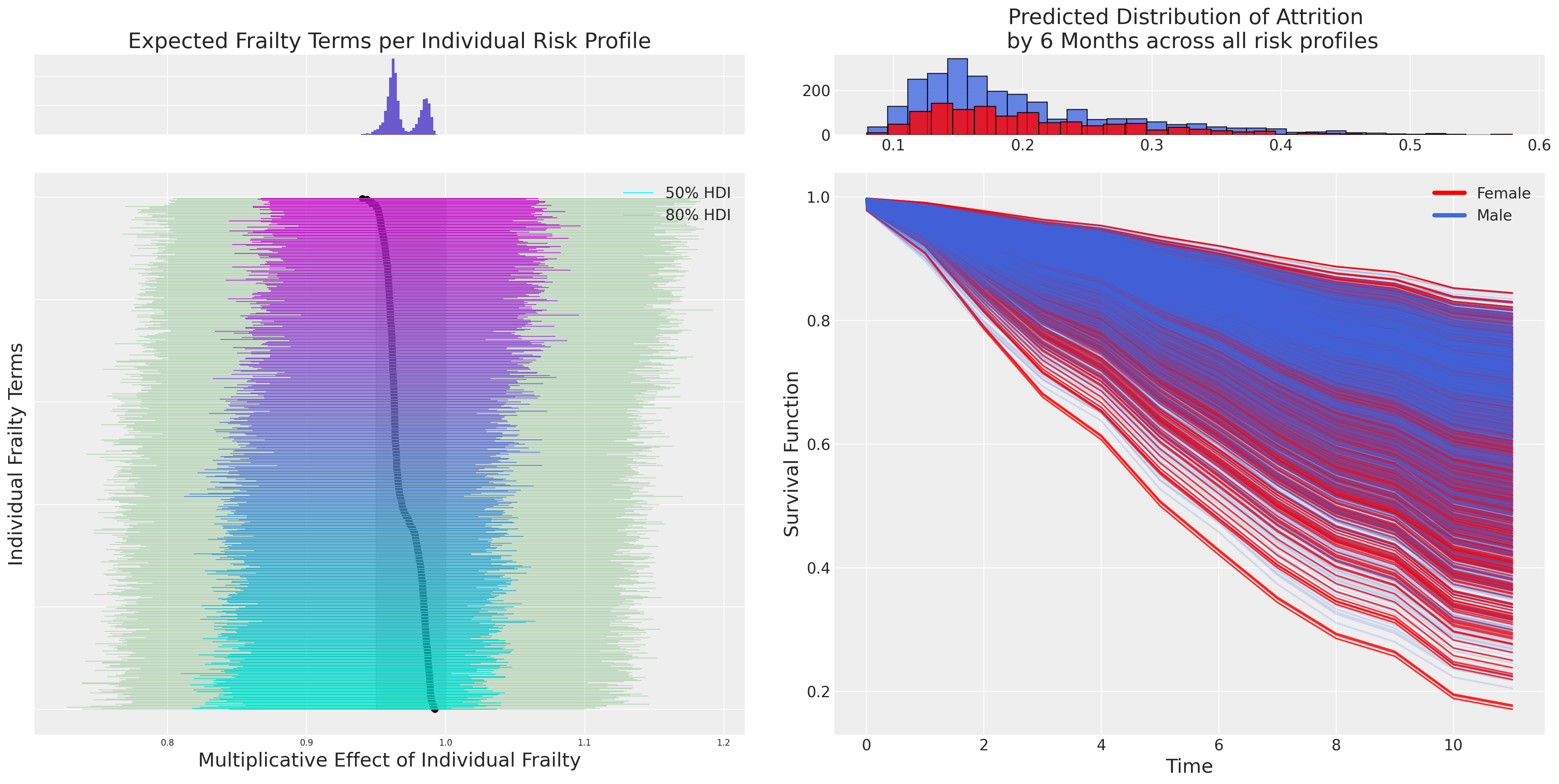
在这里，我们看到了个体脆弱项的图示以及它们对每个个体预测风险的不同乘法效应。这是一个强大的视角，用于探讨观察到的协变量对每个个体的捕捉程度以及脆弱项所暗示的调整量有多大？

结论

在这个例子中，我们看到了如何在员工生命周期中建模时间到流失的情况——我们还可能想知道为该职位招聘替代者需要多长时间！这些生存分析的应用可以在任何涉及流程效率的行业中常规应用。我们对随时间变化的风险理解得越好，我们就越能适应在高风险时期所面临的威胁。

大致上有两种观点需要平衡：(i) “精算”需求，即理解生命周期内的预期损失，以及 (ii) “诊断”需求，即理解延长或缩短生命周期的因果因素。两者最终是互补的，因为在我们为未来做计划时，需要“定价”影响预期底线的不同风险。生存回归分析巧妙地结合了这两种观点，使分析师能够理解并采取预防措施，以抵消风险增加的时期。

我们已经在上面看到了一些用于时间到事件数据的独特回归建模策略，但还有更多类型可以探索：带有生存成分的联合纵向模型、带有时间变化协变量的生存模型、治愈率模型。这些生存模型的贝叶斯视角非常有用，因为我们通常有来自前几年或实验的详细结果，我们的先验知识为问题增加了有用的视角——使我们能够将这些信息数值化，以帮助正则化复杂生存模型的拟合。在上述脆弱性模型的情况下——我们已经看到如何将先验知识添加到脆弱性项中，以描述影响个体轨迹的未观察到的协变量的影响。同样，分层方法建模基线风险使我们能够仔细表达个体风险的轨迹。这在以人为中心的学科中尤为重要，我们寻求反复测量同一个个体的数据——考虑到我们可以解释个体效应的程度。也就是说，尽管生存分析框架适用于广泛的领域和问题，但它仍然允许我们建模、预测和推断特定和个体风险方面。

作者

• 由 Nathaniel Forde 于2023年11月撰写

参考资料

[1]

大卫·科利特。医学研究中的生存数据建模。CRC出版社，2014年。

[2]

基思·麦克纳蒂。《人员分析中的回归建模手册》。查普曼和霍尔/CRC出版社，2020年。

水印

%load_ext watermark
%watermark -n -u -v -iv -w -p pytensor

Last updated: Tue Nov 28 2023

Python implementation: CPython
Python version       : 3.9.16
IPython version      : 8.11.0

pytensor: 2.11.1

matplotlib: 3.7.1
pymc      : 5.3.0
pandas    : 1.5.3
arviz     : 0.15.1
pytensor  : 2.11.1
numpy     : 1.23.5

Watermark: 2.3.1