经验近似概述#

对于大多数模型，我们使用Metropolis或NUTS等采样MCMC算法。在PyMC中，我们习惯于存储MCMC样本的轨迹，然后使用它们进行分析。PyMC中的变分推断子模块也有类似的概念：Empirical。这种近似类型为SVGD采样器存储粒子。独立SVGD粒子与MCMC样本之间没有区别。Empirical充当MCMC采样输出与apply_replacements或sample_node等全功能VI工具之间的桥梁。有关接口描述，请参见变分API快速入门。这里我们将只关注Emprical，并概述Empirical近似的特定内容。

import arviz as az
import matplotlib.pyplot as plt
import numpy as np
import pymc as pm
import pytensor
import seaborn as sns

from pandas import DataFrame

print(f"Running on PyMC v{pm.__version__}")

Running on PyMC v5.0.1

%config InlineBackend.figure_format = 'retina'
az.style.use("arviz-darkgrid")
np.random.seed(42)

多模态密度#

让我们回顾一下变分API快速入门中的问题，我们在那里首次获得了NUTS轨迹

w = pm.floatX([0.2, 0.8])
mu = pm.floatX([-0.3, 0.5])
sd = pm.floatX([0.1, 0.1])

with pm.Model() as model:
    x = pm.NormalMixture("x", w=w, mu=mu, sigma=sd)
    trace = pm.sample(50_000, return_inferencedata=False)

Auto-assigning NUTS sampler...
Initializing NUTS using jitter+adapt_diag...
Multiprocess sampling (4 chains in 4 jobs)
NUTS: [x]

100.00% [204000/204000 01:26<00:00 Sampling 4 chains, 0 divergences]

Sampling 4 chains for 1_000 tune and 50_000 draw iterations (4_000 + 200_000 draws total) took 87 seconds.

with model:
    idata = pm.to_inference_data(trace)
az.plot_trace(idata);

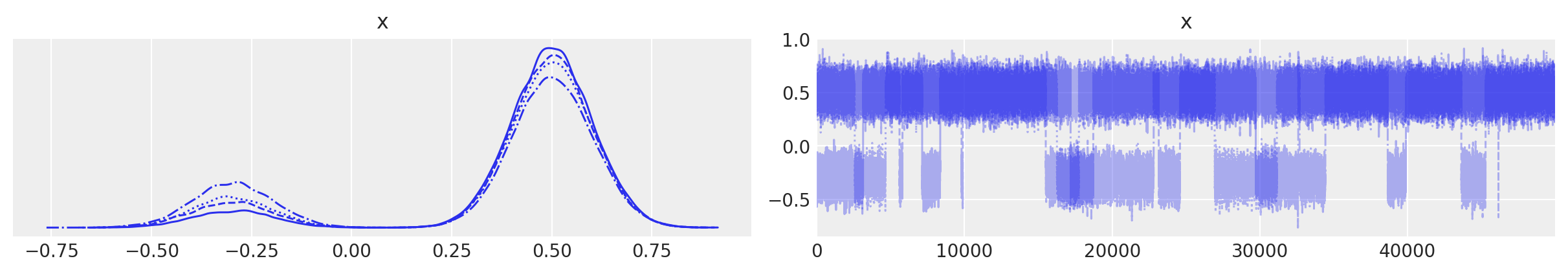
../_images/1f492e57459477c94ea1c4592c256e74214136f337eb07f676f0f5899ce5fb3e.png

太好了。首先，有了轨迹，我们可以创建 Empirical 近似

print(pm.Empirical.__doc__)

**Single Group Full Rank Approximation**

    Builds Approximation instance from a given trace,
    it has the same interface as variational approximation
    

with model:
    approx = pm.Empirical(trace)

approx

<pymc.variational.approximations.Empirical at 0x7f64b15d15b0>

这种近似方法有其自己的底层存储用于样本，即 pytensor.shared 本身

approx.histogram

histogram

approx.histogram.get_value()[:10]

array([[-0.27366748],
       [-0.32806332],
       [-0.56953621],
       [-0.2994719 ],
       [-0.18962334],
       [-0.24262214],
       [-0.36759098],
       [-0.23522732],
       [-0.37741766],
       [-0.3298074 ]])

approx.histogram.get_value().shape

(200000, 1)

它与你之前在trace中的样本数量完全相同。在我们的特定情况下，它是50k。另一个需要注意的事情是，如果你有一个包含多个链的multitrace，你将一次性存储更多的样本。我们展平所有的trace以创建Empirical。

这个直方图是关于我们如何存储样本的。结构非常简单：(n_samples, n_dim) 这些变量的顺序在类内部存储，在大多数情况下终端用户不需要使用

approx.ordering

OrderedDict([('x', ('x', slice(0, 1, None), (), dtype('float64')))])

从后验分布中进行采样是带有替换的均匀采样。调用 approx.sample(1000) 你会再次得到轨迹，但顺序是不确定的。现在无法通过 approx.sample 重建原始轨迹。

new_trace = approx.sample(50000)

采样函数编译后，采样变得非常快

az.plot_trace(new_trace);

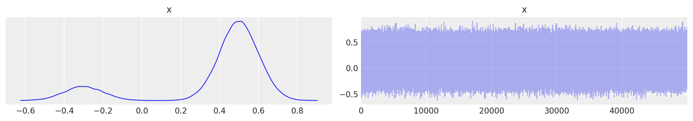
../_images/a6ff98fe105160812e9748154ee193bd35ab6c5c4976f18ae5cff8b3374218f7.png

你看到这里已经没有顺序了，但重建的密度是相同的。

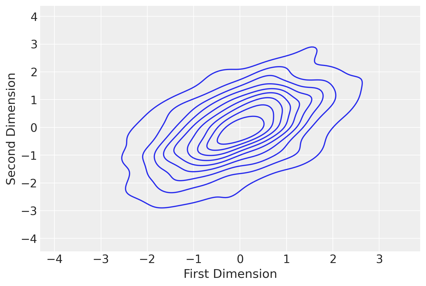
2D 密度#

mu = pm.floatX([0.0, 0.0])
cov = pm.floatX([[1, 0.5], [0.5, 1.0]])
with pm.Model() as model:
    pm.MvNormal("x", mu=mu, cov=cov, shape=2)
    trace = pm.sample(1000, return_inferencedata=False)
    idata = pm.to_inference_data(trace)

Auto-assigning NUTS sampler...
Initializing NUTS using jitter+adapt_diag...
Multiprocess sampling (4 chains in 4 jobs)
NUTS: [x]

100.00% [8000/8000 00:06<00:00 Sampling 4 chains, 0 divergences]

Sampling 4 chains for 1_000 tune and 1_000 draw iterations (4_000 + 4_000 draws total) took 7 seconds.

with model:
    approx = pm.Empirical(trace)

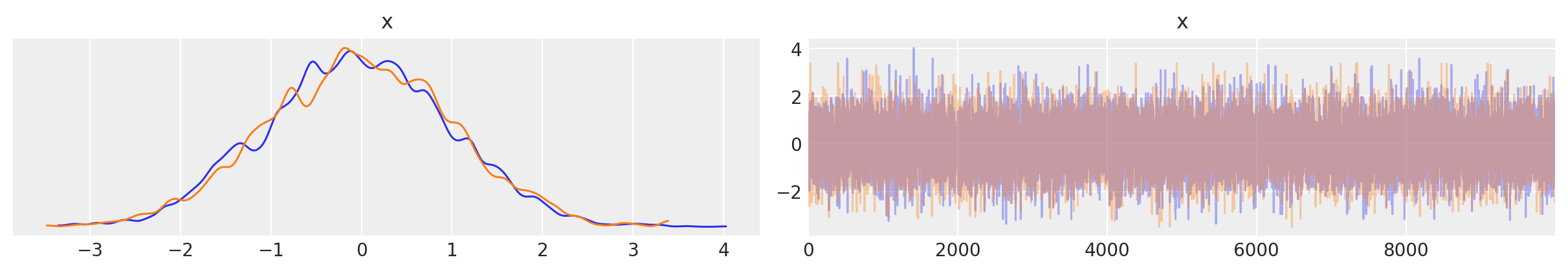
az.plot_trace(approx.sample(10000));

../_images/ab903d88091901dce5ea1151ac99457939953987cd0643419dc39f965f1bcad9.png

kdeViz_df = DataFrame(
    data=approx.sample(1000).posterior["x"].squeeze(),
    columns=["First Dimension", "Second Dimension"],
)

sns.kdeplot(data=kdeViz_df, x="First Dimension", y="Second Dimension")
plt.show()

../_images/57f01d3caf90b26ed1a392be29a6d87a4c6a6fd537f9a2650ff983fce3f1acdb.png

之前我们有一个 trace_cov 函数

with model:
    print(pm.trace_cov(trace))

[[1.04134257 0.53158646]
 [0.53158646 1.02179671]]

现在我们可以使用Empirical来估计相同的协方差

print(approx.cov)

Elemwise{true_div,no_inplace}.0

这是一个张量对象，我们需要对其进行评估。

print(approx.cov.eval())

[[1.04108223 0.53145356]
 [0.53145356 1.02154126]]

估计值非常接近，差异是由于精度误差造成的。我们可以用同样的方式得到平均值

print(approx.mean.eval())

[-0.03548692 -0.03420244]

作者#

由Maxim Kochurov撰写（pymc#2389）
由Maxim Kochurov更新（pymc#2416）
由Raul Maldonado更新（pymc-examples#21）
由 Chris Fonnesbeck 更新（pymc-examples#429）

水印#

%load_ext watermark
%watermark -n -u -v -iv -w

Last updated: Fri Jan 13 2023

Python implementation: CPython
Python version       : 3.9.0
IPython version      : 8.8.0

pymc      : 5.0.1
pytensor  : 2.8.11
arviz     : 0.14.0
sys       : 3.9.0 | packaged by conda-forge | (default, Nov 26 2020, 07:57:39) 
[GCC 9.3.0]
numpy     : 1.23.5
seaborn   : 0.12.2
matplotlib: 3.6.2

Watermark: 2.3.1

许可证声明#

本示例库中的所有笔记本均在MIT许可证下提供，该许可证允许修改和重新分发，前提是保留版权和许可证声明。

引用 PyMC 示例#

要引用此笔记本，请使用Zenodo为pymc-examples仓库提供的DOI。

重要

许多笔记本是从其他来源改编的：博客、书籍……在这种情况下，您应该引用原始来源。

同时记得引用代码中使用的相关库。

这是一个BibTeX的引用模板：

@incollection{citekey,
  author    = "<notebook authors, see above>",
  title     = "<notebook title>",
  editor    = "PyMC Team",
  booktitle = "PyMC examples",
  doi       = "10.5281/zenodo.5654871"
}

渲染后可能看起来像：

分类

标签