反事实公平性#

本文介绍并复制了Kusner等人（2018年）提出的反事实公平性，使用了DoWhy。

反事实公平性作为一种个体层面的因果公平性度量，捕捉了这样一种观念：如果一个估计器的决策在(a)现实世界和(b)个体与不同人口群体相关联的反事实世界中保持一致，则该决策被认为对个体是公平的。

何时应用反事实公平性？#

评估预测是否在个体层面上具有因果公平性，即预测对于给定个体 i 是否公平。

估计反事实公平性需要什么？#

包含受保护属性或代理变量的数据集。
结构因果模型（SCM）：通过SCM发现算法或专家驱动的因果DAG创建来发现。

符号#

A: 个人的受保护属性集合，代表不得受到歧视的变量。
a: 实际值，表示现实世界中受保护属性所取的值。
a’: 受保护属性的反事实（/翻转）值。
X: 任何特定个体的其他可观察属性。
U: 未观察到的相关潜在属性集合。
Y: 要预测的结果，可能受到历史偏见的影响。
$\hat{Y}$: 预测器，一个依赖于A、X和U的随机变量，由机器学习算法生成，作为Y的预测。

根据Pearl的定义，一个结构因果模型M被定义为一个四元组(U, V, F, P(u))，它可以用一个有向无环图(DAG)表示，其中：

U: 由模型外部因素决定的外生（未观测）变量集合。
V: 内生（观察到的）变量集合 {V1 … Vn}，完全由模型中的变量（包括 U 和 V）决定。注意：V 包括特征 X 和输出 Y。
F: 结构方程集合 {f1 … fn}，其中每个 fi 是一个过程，通过该过程 Vi 被赋予一个值 fi(v,u)，以响应 U 和 V 的当前（相关）值。
P(u): U 上的（先验）分布。
do(Zi = z): (Do) 干预 (Pearl 2000, 第3章)，表示对M的操纵，其中所选干预变量Z（V的子集）的值被设置为常量z，而不管这些值通常是如何由DAG生成的。这捕捉了一个外部代理通过强制将值z分配给Zi来修改系统的想法（例如，在随机实验中）。在公平性文献中，Z通常包括受保护的属性，如种族、性别等。

M 是因果的，因为在给定 P(U) 的情况下，对子集 Z 进行干预后，我们可以推导出 V 中剩余未干预变量的分布。

[1]:

import warnings
from collections import namedtuple
from typing import Any, Callable, Dict, List, Tuple, Union
import matplotlib.pyplot as plt
import numpy as np
import pandas as pd
from scipy import stats
import sklearn
from sklearn.neighbors import KernelDensity
from sklearn.mixture import GaussianMixture
from sklearn.linear_model import LogisticRegression, LinearRegression
from sklearn.preprocessing import LabelEncoder
from sklearn.base import BaseEstimator

import warnings
import dowhy
import matplotlib.pyplot as plt
import dowhy.gcm as gcm
import networkx as nx

from sklearn import datasets, metrics
from typing import List, Any, Union

import matplotlib.pyplot as plt
import pandas as pd
from sklearn.base import BaseEstimator


def analyse_counterfactual_fairness(
    df: pd.DataFrame,
    estimator: Union[BaseEstimator],
    protected_attrs: List[str],
    dag: List[Tuple],
    X: List[str],
    target: str,
    disadvantage_group: dict,
    intersectional: bool = False,
    return_cache: bool = False,
) -> Union[float, Tuple[float, pd.DataFrame, pd.DataFrame]]:
    """
    Calculates Counterfactual Fairness following Kusner et al. (2018)
    Reference - https://arxiv.org/pdf/1703.06856.pdf

    Args:
        df (pd.DataFrame): Pandas DataFrame containing non-factorized/dummified versions of categorical
            variables, the predicted ylabel, and other variables consumed by the predictive model.
        estimator (Union[BaseEstimator]): Predictive model to be used for generating the output.
        protected_attrs (List[str]): List of protected attributes in the dataset.
        dag (List[Tuple]): List of tuples representing the Directed Acyclic Graph (DAG) structure.
        X (List[str]): List of features to be used by the estimator.
        target (str): Name of the target variable in df.
        disadvantage_group (dict): Dictionary specifying the disadvantaged group for each protected attribute.
        intersectional (bool, optional): If True, considers intersectional fairness. Defaults to False.
        return_cache (bool, optional): If True, returns the counterfactual values with observed and
            counterfactual protected attribute interventions for each row in df. Defaults to False.

    Returns:
        counterfactual_fairness (Union[float, Tuple[float, pd.DataFrame, pd.DataFrame]]):
            - If return_cache is False, returns the calculated counterfactual fairness as a float.
            - If return_cache is True, returns a tuple containing counterfactual fairness as a float,
              DataFrame df_obs with observed counterfactual values, and DataFrame df_cf with perturbered counterfactual values.
    """

    invt_local_causal_model = gcm.InvertibleStructuralCausalModel(nx.DiGraph(dag))
    gcm.auto.assign_causal_mechanisms(invt_local_causal_model, df)

    gcm.fit(invt_local_causal_model, df)

    df_cf = pd.DataFrame()
    df_obs = pd.DataFrame()

    do_val_observed = {protected_attr: "observed" for protected_attr in protected_attrs}
    do_val_counterfact = {protected_attr: "cf" for protected_attr in protected_attrs}

    for idx, row in df.iterrows():

        do_val_obs = {}
        for protected_attr, intervention_type in do_val_observed.items():
            intervention_val = float(
                row[protected_attr]
                if intervention_type == "observed"
                else 1 - float(row[protected_attr])
            )
            do_val_obs[protected_attr] = _wrapper_lambda_fn(intervention_val)

        do_val_cf = {}
        for protected_attr, intervention_type in do_val_counterfact.items():
            intervention_val = float(
                float(row[protected_attr])
                if intervention_type == "observed"
                else 1 - float(row[protected_attr])
            )
            do_val_cf[protected_attr] = _wrapper_lambda_fn(intervention_val)

        counterfactual_samples_obs = gcm.counterfactual_samples(
            invt_local_causal_model, do_val_obs, observed_data=pd.DataFrame(row).T
        )

        counterfactual_samples_cf = gcm.counterfactual_samples(
            invt_local_causal_model, do_val_cf, observed_data=pd.DataFrame(row).T
        )

        df_cf = pd.concat([df_cf, counterfactual_samples_cf])
        df_obs = pd.concat([df_obs, counterfactual_samples_obs])

    df_cf = df_cf.reset_index(drop=True)
    df_obs = df_obs.reset_index(drop=True)

    if hasattr(estimator, "predict_proba"):
        # 1. Samples from the causal model based on the observed race
        lr_observed = estimator()
        lr_observed.fit(df_obs[X].astype(float), df[target])
        df_obs[f"preds"] = lr_observed.predict_proba(df_obs[X].astype(float))[:, 1]

        # 2. Samples from the causal model based on the counterfactual race
        lr_cf = estimator()
        lr_cf.fit(df_cf[X].astype(float), df[target])
        df_cf[f"preds_cf"] = lr_cf.predict_proba(df_cf[X].astype(float))[:, 1]

    else:
        # 1. Samples from the causal model based on the observed race
        lr_observed = estimator()
        lr_observed.fit(df_obs[X].astype(float), df[target])
        df_obs[f"preds"] = lr_observed.predict(df_obs[X].astype(float))

        # 2. Samples from the causal model based on the counterfactual race
        lr_cf = estimator()
        lr_cf.fit(df_cf[X].astype(float), df[target])
        df_cf[f"preds_cf"] = lr_cf.predict(df_cf[X].astype(float))

    query = " and ".join(
        f"{protected_attr} == {disadvantage_group[protected_attr]}"
        for protected_attr in protected_attrs
    )
    mask = df.query(query).index.tolist()
    counterfactual_fairness = (
        df_obs.loc[mask]["preds"].mean() - df_cf.loc[mask]["preds_cf"].mean()
    )

    if not return_cache:
        return counterfactual_fairness
    else:
        return counterfactual_fairness, df_obs, df_cf

def plot_counterfactual_fairness(
    df_obs: pd.DataFrame,
    df_cf: pd.DataFrame,
    mask: pd.Series,
    counterfactual_fairness: Union[int, float],
    legend_observed: str,
    legend_counterfactual: str,
    target: str,
    title: str,
) -> None:
    """
    Plots counterfactual fairness comparing observed and counterfactual samples.

    Args:
        df_obs (pd.DataFrame): DataFrame containing observed samples.
        df_cf (pd.DataFrame): DataFrame containing counterfactual samples.
        mask (pd.Series): Boolean mask for selecting specific samples from the DataFrames.
        counterfactual_fairness (Union[int, float]): The counterfactual fairness metric.
        legend_observed (str): Legend label for the observed samples.
        legend_counterfactual (str): Legend label for the counterfactual samples.
        target (str): Name of the target variable to be plotted on the x-axis.
        title (str): Title of the plot.

    Returns:
        None: The function displays the plot.
    """

    fig, ax = plt.subplots(figsize=(8, 5), nrows=1, ncols=1)

    ax.hist(
        df_obs[f"preds"][mask], bins=50, alpha=0.7, label=legend_observed, color="blue"
    )
    ax.hist(
        df_cf[f"preds_cf"][mask], bins=50, alpha=0.7, label=legend_counterfactual, color="orange"
    )

    ax.set_xlabel(target)
    ax.legend()
    ax.set_title(title)

    fig.suptitle(f"Counterfactual Fairness {round(counterfactual_fairness, 3)}")

    plt.tight_layout()
    plt.show()


def _wrapper_lambda_fn(val):
    return lambda x: val

1. 加载并清理数据集#

Kusner等人（2018年）使用了一项由法学院入学委员会进行的调查，涵盖了美国163所法学院，收集了21,790名法学院学生的数据。本案例研究中使用的最初数据集是为Linda Wightman在1998年进行的一项名为‘LSAC国家纵向律师资格考试研究。LSAC研究报告系列’的研究而收集的。该调查包括以下详细信息：- 入学考试成绩（LSAT）- 法学院前的平均绩点（GPA）- 第一年的平均成绩（FYA）。

它还包括受保护的属性，例如：- 种族 - 性别

为了本示例的目的，我们将仅关注白人和黑人亚组之间的结果差异，并将数据集限制为5000个个体的随机样本：

[2]:

df = pd.read_csv("datasets/law_data.csv")

df["Gender"] = df["sex"].map({2: 0, 1: 1}).astype(str)
df["Race"] = df["race"].map({"White": 0, "Black": 1}).astype(str)

df = (
    df.query("race=='White' or race=='Black'")
    .rename(columns={"UGPA": "GPA", "LSAT": "LSAT", "ZFYA": "avg_grade"})[
        ["Race", "Gender", "GPA", "LSAT", "avg_grade"]
    ]
    .reset_index(drop=True)
)

df_sample = df.astype(float).sample(5000).reset_index(drop=True)

df_sample.head()

[2]:

	种族	性别	GPA	LSAT	平均成绩
0	0.0	0.0	3.9	45.0	0.62
1	0.0	1.0	3.6	48.0	1.71
2	0.0	1.0	3.0	32.0	0.20
3	0.0	0.0	3.8	41.0	1.26
4	1.0	1.0	2.9	35.0	-1.28

根据这些数据，学校可能希望预测申请人是否会有较高的FYA。学校还希望确保这些预测不会因个人的种族和性别而产生偏见。然而，LSAT、GPA和FYA分数可能由于社会因素而产生偏见。那么，我们如何确定这种预测模型对特定个人的偏见程度呢？使用反事实公平性。

2. 反事实公平性的正式定义#

反事实公平性要求，对于人群中的每个人，即使在因果意义上该人具有不同的受保护属性，预测值也应保持不变。更正式地说，$\hat{Y}$ 在任何上下文 X = x 和 A = a 下都是反事实公平的：

\[P(\hat{Y}_{a}(U) = y | X = x, A = a) = P(\hat{Y}_{a'}(U) = y | X = x, A = a)\]

对于所有y和A可达到的任何值a'。这个概念与实际原因或标记因果关系密切相关。本质上，为了公平性，A不应是$\hat{Y}$在任何特定实例中的直接原因，即在保持非因果依赖因素不变的情况下改变A不应改变$\hat{Y}$的分布。对于个体i，从各种反事实世界生成的Y之间的差异可以理解为相似性的度量。

2.1 测量反事实公平性#

在一个SCM M中，任何可观察变量（Vi）的状态完全由背景变量（U）和结构方程（F）决定。因此，给定一组完全指定的方程，我们可以使用SCM构建反事实。也就是说

"we can compute what (the distribution of) any of the variables would have been had certain other variables been different, other things being equal. For instance, given the causal model we can ask “Would individual i have graduated (Y = 1) if they hadn’t had a job?”, even if they did not actually graduate in the dataset." - (Russell et. al. , 2017)

给定一个SCM M和证据E（V的子集），反事实通过三个步骤构建（即推断）：

反演: 即使用模型M，调整噪声变量以与观察到的证据E一致。更正式地说，给定E和先验分布P(U)，计算给定M的未观察变量集U的值。对于非确定性模型（如文献中的大多数因果模型），计算后验分布P(U|E=e)。
操作: 对 Z 执行 do-intervention（即 do(Zi = z)），从而得到干预后的 SCM 模型 M’。
预测: 使用干预后的模型 M’ 和 P(U|E=e)，计算 V 的反事实值（或 P(V |E=e)）。

3. 使用DoWhy测量反事实公平性#

从算法上讲，要经验性地测试一个模型是否具有反事实公平性：

步骤1 - 定义一个因果模型 基于因果DAG
步骤2 - 生成反事实样本: 使用 gcm.counterfactual_samples ，从模型中生成两组样本：
1. 一组使用受保护属性的观察值 (df_obs)
2. 一组使用受保护属性的反事实值 (df_cf)
步骤 3 - 使用采样数据拟合估计器: 将模型拟合到原始和反事实的采样数据上，并绘制由两个模型生成的预测目标的分布图。如果分布重叠，则估计器在反事实上是公平的，否则不是。

给定一个包含受保护/代理属性和因果DAG的数据集，我们可以使用analyse_counterfactual_fairness函数来测量个体和总体层面的反事实公平性。在这个例子中，我们基于Kusner等人（2018）提供的因果DAG创建了因果DAG。

[3]:

dag = [
    ("Race", "GPA"),
    ("Race", "LSAT"),
    ("Race", "avg_grade"),
    ("Gender", "GPA"),
    ("Gender", "LSAT"),
    ("Gender", "avg_grade"),
    ("GPA", "avg_grade"),
    ("LSAT", "avg_grade"),
]

analyse_counterfactual_fairness 方法还接受以下输入：- 目标变量的名称（此处为 target，即 avg_grade）- 输入数据集（df）- 一个未拟合的 sklearn 估计器（estimator；此处为 LinearRegression）- 受保护属性列表（protected_attrs）- 输入特征名称列表（X）- 一个字典，指定每个受保护群体中弱势群体的唯一标识标签（disadvantage_group）。

[4]:

target = "avg_grade"
disadvantage_group = {"Race": 1}
protected_attrs = ["Race"]
features = ["GPA", "LSAT"]

3.1 单变量分析#

现在，我们准备调用方法 analyse_counterfactual_fairness 来沿着种族维度进行反事实公平性分析：

[5]:

config = {
    "df": df_sample,
    "dag": dag,
    "estimator": LinearRegression,
    "protected_attrs": protected_attrs,
    "X": features,
    "target": target,
    "disadvantage_group": disadvantage_group,
    "return_cache": True,
}

counterfactual_fairness, df_obs, df_cf = analyse_counterfactual_fairness(**config)
counterfactual_fairness

Fitting causal mechanism of node Gender: 100%|██████████| 5/5 [00:00<00:00, 55.16it/s]

[5]:

$\displaystyle -0.501612555470459$

df_obs 包含每个个体在现实世界中其受保护属性观察值下的预测值。

[6]:

df_obs.head()

[6]:

	种族	性别	平均绩点	法学院入学考试	平均成绩	预测
0	0.0	0.0	3.9	45.0	0.62	0.646472
1	0.0	1.0	3.6	48.0	1.71	0.685566
2	0.0	1.0	3.0	32.0	0.20	-0.132365
3	0.0	0.0	3.8	41.0	1.26	0.455839
4	1.0	1.0	2.9	35.0	-1.28	-0.037868

df_cf 包含了在现实世界中每个个体在受保护属性的反事实值下的预测值。在这里，由于我们干预的唯一变量是种族，我们看到每个个体的种族已从0更改为1。

[7]:

df_cf.head()

[7]:

	种族	性别	GPA	LSAT	平均成绩	预测值_cf
0	1.0	0.0	3.577589	37.124987	-0.918331	0.278384
1	1.0	1.0	3.203434	40.124987	0.425989	0.263249
2	1.0	1.0	2.603434	24.124987	-0.579415	0.048368
3	1.0	0.0	3.477589	33.124987	-0.170558	0.230359
4	0.0	1.0	3.296566	42.875013	-0.204968	0.299043

[8]:

plot_counterfactual_fairness(
    df_obs=df_obs,
    df_cf=df_cf,
    mask=(df_sample["Race"] == 1).values,
    counterfactual_fairness=counterfactual_fairness,
    legend_observed="Observed Samples (Race=Black)",
    legend_counterfactual="Counterfactual Samples (Race=White)",
    target=target,
    title="Black -> White",
)

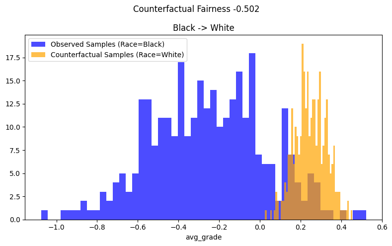
../_images/example_notebooks_counterfactual_fairness_dowhy_16_0.png

检查图1中的示例结果，我们观察到观察到的分布和反事实分布没有重叠。我们发现，将黑人子组的种族更改为白人子组会使$\hat{Y}$的分布向右移动，即平均将avg_grade增加约0.50。因此，可以得出结论，拟合的估计器在反事实上是不公平的。

3.2 交叉分析#

我们可以进一步从交叉性的角度扩展分析，通过一起检查多个受保护属性对反事实公平性的影响。在这里，我们使用我们可用的两个受保护属性 - ["Race","Gender"] - 来进行交叉反事实公平性分析，以确定估计器对黑人女性的反事实公平性如何：

[9]:

disadvantage_group = {"Race": 1, "Gender": 1}
config = {
    "df": df_sample.astype(float).reset_index(drop=True),
    "estimator": LinearRegression,
    "protected_attrs": ["Race", "Gender"],
    "dag": dag,
    "X": features,
    "target": "avg_grade",
    "return_cache": True,
    "disadvantage_group": disadvantage_group,
    "intersectional": True,
}

counterfactual_fairness, df_obs, df_cf = analyse_counterfactual_fairness(**config)
counterfactual_fairness

Fitting causal mechanism of node Gender: 100%|██████████| 5/5 [00:00<00:00, 78.72it/s]

[9]:

$\displaystyle -0.504504518545456$

[10]:

plot_counterfactual_fairness(
    df_obs=df_obs,
    df_cf=df_cf,
    mask=((df_sample["Race"] == 1).values & (df_sample["Gender"] == 1).values),
    counterfactual_fairness=counterfactual_fairness,
    legend_observed="Observed Samples (Race=Black, Gender=Female)",
    legend_counterfactual="Counterfactual Samples (Race=White, Gender=Male)",
    target=target,
    title="(Black, Female) -> (White, Male)",
)

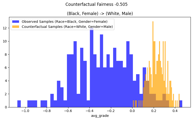
../_images/example_notebooks_counterfactual_fairness_dowhy_19_0.png

通过分析图2中的交叉分析结果，我们发现观察到的分布和反事实分布完全没有重叠。将黑人女性的种族和性别改为白人男性，会使黑人女性子组的$\hat{Y}$分布向右移动，即平均将avg_grade提高约0.50。因此，可以得出结论，拟合的估计器在交叉情况下不具有反事实公平性。

3.3 反事实的额外用途 `df_obs` , `df_cf` 用于公平性#

在存在历史偏见标签Y的情况下，Y的反事实值（使用一组公平因果模型构建）可以用作训练模型的公平目标。
通过使用一种优化例程来训练一个估计器，使其在反事实世界中对于给定个体i的Y（平均）差异成比例地施加惩罚，从而实现反事实公平。例如，如果对于个体i，在反事实世界中结果Y差异很大，那么该样本i将按比例增加损失。相反，如果对于个体j，在反事实世界中结果Y相似，那么该样本i将按比例减少损失（更多详情请参见Russell, Chris等人，2017）。

4. 反事实公平性的限制#

关于“正确的”因果模型可能存在分歧，原因如下：

更改DAG的结构，例如添加边
改变潜在变量，例如改变生成节点的函数以具有不同的信号与噪声分解
防止某些路径传播反事实值

文献建议在多个竞争的因果模型下实现反事实公平性作为上述问题的解决方案。Russell等人（2017）提出了一个名为“多世界公平算法”的解决方案。

参考文献#

Kusner, Matt 等人. 反事实公平性. 2018, https://arxiv.org/pdf/1703.06856.pdf
Russell, Chris 等人。当世界碰撞时：在公平性中整合不同的反事实假设。2017年，https://proceedings.neurips.cc/paper/2017/file/1271a7029c9df08643b631b02cf9e116-Paper.pdf

附录：通过无意识实现的公平性（FTU）创建了一个反事实不公平的估计器#

为了证明“Aware”线性回归总是反事实公平的，但FTU使其反事实不公平，我们构建了一个“aware”线性回归，并将其与图1中构建的“unaware”线性回归进行比较。

[11]:

config = {
    "df": df_sample,
    "estimator": LinearRegression,
    "protected_attrs": ["Race"],
    "dag": dag,
    "X": ["GPA", "LSAT", "Race", "Gender"],
    "target": "avg_grade",
    "return_cache": True,
    "disadvantage_group": disadvantage_group,
}

counterfactual_fairness_aware, df_obs_aware, df_cf_aware = (
    analyse_counterfactual_fairness(**config)
)
counterfactual_fairness_aware

Fitting causal mechanism of node Gender: 100%|██████████| 5/5 [00:00<00:00, 63.95it/s]

[11]:

$\displaystyle 5.55111512312578 \cdot 10^{-16}$

[12]:

plot_counterfactual_fairness(
    df_obs=df_obs_aware,
    df_cf=df_cf_aware,
    mask=(df_sample["Race"] == 1).values,
    counterfactual_fairness=counterfactual_fairness_aware,
    legend_observed="Observed Samples (Race=Black)",
    legend_counterfactual="Counterfactual Samples (Race=White)",
    target=target,
    title="Black -> White",
)

../_images/example_notebooks_counterfactual_fairness_dowhy_23_0.png

比较图1和图3，观察到的反事实样本 df_obs 和扰动的反事实样本 df_cf 的比较图显示：

对于图3中的“aware”线性回归，两个分布重叠。因此，估计器是反事实公平的。
对于图1中的“无意识”线性回归，两个分布非常不同且不重叠，这表明估计器在反事实上是公平的，即仅将avg_grade回归到GPA和LSAT上会使估计器在反事实上不公平。

值得注意的是，可以正式证明，通常情况下，“仅对Y进行X回归符合FTU标准，但并不具有反事实公平性，因此省略A（FTU）可能会在一个原本公平的世界中引入不公平性”。（Kusner等，2018年）