401(k)资格对净金融资产的影响#
在本案例研究中,我们将使用来自401(k)分析的真实数据来解释如何使用图形因果模型来估计平均处理效应(ATE)和条件平均处理效应(CATE)。
背景#
在20世纪80年代初,美国政府为员工推出了几种税收递延储蓄选项,以增加个人退休储蓄。一个受欢迎的选择是401(k)计划,该计划允许员工将一部分工资存入个人账户。这里的目的是了解401(k)资格对净金融资产(即401(k)余额和非401(k)资产的总和)的影响,考虑到由于个人特征(特别是收入)导致的异质性。
由于401(k)计划由雇主提供,只有提供这些计划的公司的员工才有资格参与。因此,我们正在处理一项非随机研究。有几个因素(例如教育、储蓄偏好)会影响401(k)的资格以及净金融资产。
数据#
我们考虑1991年收入与计划参与调查中的一个样本。该样本由家庭组成,其中参考个体年龄在25-64岁之间,且至少有一人就业但无人自雇。样本中有9915户家庭的记录。对于每个家庭,记录了44个变量,包括家庭参考人是否有资格参加401(k)计划(处理变量)、净金融资产(结果变量)以及其他协变量,如年龄、收入、家庭规模、教育程度、婚姻状况等。我们特别考虑了16个协变量。
我们在下表中总结了用于本案例研究的变量。
变量名称 |
类型 |
详情 |
|---|---|---|
e401 |
处理 |
401(k)计划的资格 |
net_tfa |
结果 |
净金融资产(以美元计) |
age |
协变量 |
年龄 |
inc |
协变量 |
收入(以美元计) |
fsize |
协变量 |
家庭规模 |
educ |
协变量 |
教育(以年为单位) |
男性 |
协变量 |
是男性吗? |
db |
协变量 |
确定给付养老金 |
marr |
协变量 |
已婚? |
twoearn |
协变量 |
双收入者 |
pira |
协变量 |
参与IRA |
hown |
协变量 |
房主? |
hval |
协变量 |
房屋价值(以美元计) |
hequity |
协变量 |
家庭资产净值(以美元计) |
hmort |
协变量 |
家庭抵押贷款(以美元计) |
nohs |
协变量 |
没有高中?(独热编码) |
hs |
协变量 |
高中?(独热编码) |
smcol |
协变量 |
是否上过大学?(独热编码) |
该数据集可从`hdm <https://rdrr.io/cran/hdm/man/pension.html>`__ R包在线公开获取。有关数据集的更多详细信息,我们建议感兴趣的读者参考以下论文:
Chernohukov, C. Hansen (2004). 401(k)参与对财富分配的影响:一种工具变量分位数回归分析. 经济与统计评论 86 (3), 735–751.
让我们先加载并分析数据。
[1]:
import pandas as pd
df = pd.read_csv("pension.csv")
[2]:
df.head()
[2]:
| ira | a401 | hval | hmort | hequity | nifa | net_nifa | tfa | net_tfa | tfa_he | ... | i3 | i4 | i5 | i6 | i7 | a1 | a2 | a3 | a4 | a5 | |
|---|---|---|---|---|---|---|---|---|---|---|---|---|---|---|---|---|---|---|---|---|---|
| 0 | 0 | 0 | 69000 | 60150 | 8850 | 100 | -3300 | 100 | -3300 | 5550 | ... | 1.0 | 0.0 | 0.0 | 0.0 | 0.0 | 0.0 | 1.0 | 0.0 | 0.0 | 0.0 |
| 1 | 0 | 0 | 78000 | 20000 | 58000 | 61010 | 61010 | 61010 | 61010 | 119010 | ... | 0.0 | 1.0 | 0.0 | 0.0 | 0.0 | 0.0 | 0.0 | 0.0 | 1.0 | 0.0 |
| 2 | 1800 | 0 | 200000 | 15900 | 184100 | 7549 | 7049 | 9349 | 8849 | 192949 | ... | 0.0 | 0.0 | 0.0 | 1.0 | 0.0 | 0.0 | 0.0 | 0.0 | 1.0 | 0.0 |
| 3 | 0 | 0 | 0 | 0 | 0 | 2487 | -6013 | 2487 | -6013 | -6013 | ... | 0.0 | 0.0 | 1.0 | 0.0 | 0.0 | 1.0 | 0.0 | 0.0 | 0.0 | 0.0 |
| 4 | 0 | 0 | 300000 | 90000 | 210000 | 10625 | -2375 | 10625 | -2375 | 207625 | ... | 0.0 | 1.0 | 0.0 | 0.0 | 0.0 | 0.0 | 0.0 | 1.0 | 0.0 | 0.0 |
5 行 × 44 列
401(k)资格对净金融资产的影响,基于收入条件#
首先,我们构建了一个关于401(k)计划资格(处理\(T\))、净金融资产(结果\(Y\))、控制变量\(W\)(我们假设它们阻断了\(Y\)和\(T\)之间的所有后门路径)以及收入\(X\)(基于此我们想要研究处理效果的异质性的协变量)的因果图。
[3]:
import networkx as nx
import dowhy.gcm as gcm

treatment_var = "e401"
outcome_var = "net_tfa"
covariates = ["age","inc","fsize","educ","male","db",
              "marr","twoearn","pira","hown","hval",
              "hequity","hmort","nohs","hs","smcol"]

edges = [(treatment_var, outcome_var)]
edges.extend([(covariate, treatment_var) for covariate in covariates])
edges.extend([(covariate, outcome_var) for covariate in covariates])

# To ensure that the treatment is considered as a categorical variable, we convert the values explicitly to strings.
df = df.astype({treatment_var: str})

causal_graph = nx.DiGraph(edges)
[4]:
from dowhy.utils import plot

plot(causal_graph, figure_size=[20, 20])
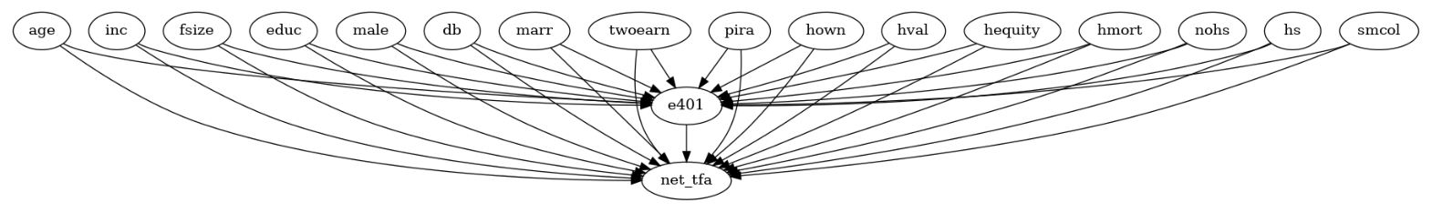
在这里,我们创建了一个简化的图,其中协变量之间没有相互作用(即\(X \cup W\)中的节点)。在实际情况中,这很可能不是这样。然而,当我们从观察数据中直接获取协变量的联合样本以估计CATEs时,我们可以忽略它们之间的相互作用。
在我们为变量分配因果模型之前,让我们绘制它们的直方图以了解变量的分布情况。
[5]:
import matplotlib.pyplot as plt

cols = [treatment_var, outcome_var]
cols.extend(covariates)
plt.figure(figsize=(10,5))
for i, col in enumerate(cols):
    plt.subplot(3,6,i+1)
    plt.grid(False)
    plt.hist(df[col])
    plt.xlabel(col)
plt.tight_layout()
plt.show()
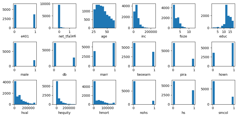
我们观察到实值变量并不遵循像高斯分布这样的知名参数分布。因此,当这些变量没有父节点时,我们拟合经验分布,这也适用于分类变量。
让我们明确地为每个节点分配因果机制。对于处理变量,我们分配一个带有随机森林分类器的分类器功能因果模型(FCM)。对于结果变量,我们分配一个带有随机森林回归作为函数和噪声的经验分布的加性噪声模型。我们为其他变量分配经验分布,因为它们在因果图中没有父节点。
[6]:
causal_model = gcm.StructuralCausalModel(causal_graph)
causal_model.set_causal_mechanism(treatment_var, gcm.ClassifierFCM(gcm.ml.create_random_forest_classifier()))
causal_model.set_causal_mechanism(outcome_var, gcm.AdditiveNoiseModel(gcm.ml.create_random_forest_regressor()))
for covariate in covariates:
    causal_model.set_causal_mechanism(covariate, gcm.EmpiricalDistribution())
如果我们没有先验知识或不熟悉统计含义,我们也可以使用启发式方法自动分配因果机制:
gcm.auto.assign_causal_mechanisms(causal_model, df)
这样,我们现在可以从数据中学习因果模型。
[7]:
gcm.fit(causal_model, df)
Fitting causal mechanism of node smcol: 100%|██████████| 18/18 [00:06<00:00, 2.67it/s]
在计算CATE之前,我们首先将家庭按收入百分位数划分为等宽区间。这使我们能够研究对不同收入群体的影响。
[8]:
import numpy as np

percentages = [0.0, 0.2, 0.4, 0.6, 0.8, 1.0]
bin_edges = [0]
bin_edges.extend(np.quantile(df.inc, percentages[1:]).tolist())
bin_edges[-1] += 1 # adding 1 to the last edge as last edge is excluded by np.digitize

groups = [f'{percentages[i]*100:.0f}%-{percentages[i+1]*100:.0f}%' for i in range(len(percentages)-1)]
group_index_to_group_label = dict(zip(range(1, len(bin_edges)+1), groups))
现在我们可以计算CATE。为此,我们在拟合的因果图中对治疗变量进行随机干预,从干预分布中抽取样本,按收入组对观察结果进行分组,然后计算每组的治疗效果。
[9]:
np.random.seed(47)

def estimate_cate():
    samples = gcm.interventional_samples(causal_model,
                                         {treatment_var: lambda x: np.random.choice(['0', '1'])},
                                         observed_data=df)
    eligible = samples[treatment_var] == '1'
    ate = samples[eligible][outcome_var].mean() - samples[~eligible][outcome_var].mean()
    result = dict(ate = ate)

    group_indices = np.digitize(samples['inc'], bin_edges)
    samples['group_index'] = group_indices

    for group_index in group_index_to_group_label:
        group_samples = samples[samples['group_index'] == group_index]
        eligible_in_group = group_samples[treatment_var] == '1'
        cate = group_samples[eligible_in_group][outcome_var].mean() - group_samples[~eligible_in_group][outcome_var].mean()
        result[group_index_to_group_label[group_index]] = cate

    return result

group_to_median, group_to_ci = gcm.confidence_intervals(estimate_cate, num_bootstrap_resamples=100)
print(group_to_median)
print(group_to_ci)
Estimating bootstrap interval...: 100%|██████████| 100/100 [00:43<00:00, 2.32it/s]
{'ate': 6524.583223183401, '0%-20%': 4010.8760624539045, '20%-40%': 3124.591365845997, '40%-60%': 5479.491988474934, '60%-80%': 7622.045252631407, '80%-100%': 12235.611495154653}
{'ate': array([4912.93938262, 8465.43365925]), '0%-20%': array([2612.44786522, 5582.21766875]), '20%-40%': array([1187.57446995, 5164.17566841]), '40%-60%': array([3333.67563274, 8129.58879172]), '60%-80%': array([ 4696.03425313, 10738.80810366]), '80%-100%': array([ 5083.79029031, 18774.95557817])}
401(k)资格对净金融资产的平均治疗效果是积极的,正如相应的置信区间所示。现在,让我们绘制不同收入组的CATEs以获得清晰的图像。
[10]:
fig = plt.figure(figsize=(8,4))
for x, group in enumerate(groups):
    ci = group_to_ci[group]
    plt.plot((x, x), (ci[0], ci[1]), 'ro-', color='orange')
ax = fig.axes[0]
ax.spines['right'].set_visible(False)
ax.spines['top'].set_visible(False)
plt.xticks(range(len(groups)), groups)
plt.xlabel('Income group')
plt.ylabel('ATE of 401(k) eligibility on net financial assets')
plt.show()
/tmp/ipykernel_4333/1344202636.py:4: UserWarning: color is redundantly defined by the 'color' keyword argument and the fmt string "ro-" (-> color='r'). The keyword argument will take precedence.
  plt.plot((x, x), (ci[0], ci[1]), 'ro-', color='orange')
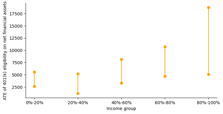
随着收入群体从低到高,影响逐渐增加。这一结果似乎与不同收入群体的资源限制相一致。