估计现实世界示例中的内在因果影响

本笔记本演示了如何使用内在因果影响（ICC）方法，这是一种估计系统中因果影响的方法。在许多应用中，一个常见的问题是：“节点X对节点Y的因果影响是什么？”在这里，“因果影响”可以通过多种方式定义。一种方法可能是测量干预影响，即“如果我对节点X进行干预，节点Y会改变多少？”或者从特征相关性的角度来看，“X在描述Y时有多相关？”

在以下内容中，我们专注于一种特定类型的因果影响，这种影响基于将生成过程分解为每个节点上的机制，并由相应的因果机制形式化。然后，ICC为每个节点量化可以追溯到相应机制的目标不确定性量。因此，从其父节点确定性计算的节点获得零贡献。这个概念最初可能看起来很复杂，但它基于一个简单的想法：

考虑一个节点链：X -> Y -> Z。Y 比 X 更能提供关于 Z 的信息，因为 Y 直接决定了 Z，并且还包含了来自 X 的所有信息。显然，当对 X 或 Y 进行干预时，Y 对 Z 的影响更大。但是，如果 Y 只是 X 的重新缩放副本，即 \(Y = a \cdot X\) 呢？在这种情况下，Y 仍然对 Z 具有最大的干预影响，但它并没有在 X 的基础上添加任何新信息。另一方面，ICC 方法会将 Y 的影响归为 0，因为它只传递了从 X 继承的内容。

ICC背后的思想不是估计观察到的上游节点对目标节点的贡献，而是归因于它们的噪声项的影响。由于我们将每个节点建模为形式为\(X_i = f_i(PA_i, N_i)\)的函数因果模型，我们的目标是估计\(N_i\)项对目标的贡献。在前面的例子中，我们有零噪声的确定性关系，即内在影响为0。这种类型的归因只有在我们明确使用函数因果模型建模因果关系时才有可能，就像我们在GCM模块中所做的那样。

在下面，我们将看两个实际例子，我们在其中应用了ICC。

汽车MPG消耗的内在影响

在第一个示例中，我们使用了著名的MPG数据集，该数据集包含用于预测汽车发动机每加仑英里数（mpg）的不同特征。假设我们的任务是改进设计过程，我们需要深入了解变量对mpg消耗的影响。这些特征之间的关系可以建模为图形因果模型。为此，我们遵循Wang等人的工作中定义的因果图，并移除所有对MPG没有影响的节点。这给我们留下了以下图形：

import pandas as pd
import networkx as nx
import numpy as np

from dowhy import gcm
from dowhy.utils.plotting import plot, bar_plot
gcm.util.general.set_random_seed(0)

# Load a modified version of the Auto MPG data: Quinlan,R.. (1993). Auto MPG. UCI Machine Learning Repository. https://doi.org/10.24432/C5859H.
auto_mpg_data = pd.read_csv("datasets/auto_mpg.csv", index_col=0)

mpg_graph = nx.DiGraph([('cylinders', 'displacement'),
                        ('cylinders', 'displacement'),
                        ('displacement', 'weight'),
                        ('displacement', 'horsepower'),
                        ('weight', 'mpg'),
                        ('horsepower', 'mpg')])

plot(mpg_graph)

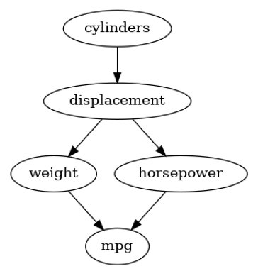
看到这个图表，我们可以预期节点之间存在一些强混杂因素，但尽管如此，我们将会看到ICC方法仍然提供了非平凡的见解。

让我们定义相应的结构因果模型并将其拟合到数据中：

scm_mpg = gcm.StructuralCausalModel(mpg_graph)
gcm.auto.assign_causal_mechanisms(scm_mpg, auto_mpg_data)
gcm.fit(scm_mpg, auto_mpg_data)

Fitting causal mechanism of node mpg: 100%|██████████| 5/5 [00:00<00:00, 30.05it/s]

可选地，我们可以通过使用评估方法来深入了解因果机制的性能：

print(gcm.evaluate_causal_model(scm_mpg, auto_mpg_data, evaluate_invertibility_assumptions=False, evaluate_causal_structure=False))

Evaluating causal mechanisms...: 100%|██████████| 5/5 [00:00<00:00, 5281.17it/s]

Evaluated the performance of the causal mechanisms and the overall average KL divergence between generated and observed distribution. The results are as follows:

==== Evaluation of Causal Mechanisms ====
The used evaluation metrics are:
- KL divergence (only for root-nodes): Evaluates the divergence between the generated and the observed distribution.
- Mean Squared Error (MSE): Evaluates the average squared differences between the observed values and the conditional expectation of the causal mechanisms.
- Normalized MSE (NMSE): The MSE normalized by the standard deviation for better comparison.
- R2 coefficient: Indicates how much variance is explained by the conditional expectations of the mechanisms. Note, however, that this can be misleading for nonlinear relationships.
- F1 score (only for categorical non-root nodes): The harmonic mean of the precision and recall indicating the goodness of the underlying classifier model.
- (normalized) Continuous Ranked Probability Score (CRPS): The CRPS generalizes the Mean Absolute Percentage Error to probabilistic predictions. This gives insights into the accuracy and calibration of the causal mechanisms.
NOTE: Every metric focuses on different aspects and they might not consistently indicate a good or bad performance.
We will mostly utilize the CRPS for comparing and interpreting the performance of the mechanisms, since this captures the most important properties for the causal model.

--- Node cylinders
- The KL divergence between generated and observed distribution is 0.0.
The estimated KL divergence indicates an overall very good representation of the data distribution.

--- Node displacement
- The MSE is 1038.9343497781185.
- The NMSE is 0.3099451012063349.
- The R2 coefficient is 0.902742668556819.
- The normalized CRPS is 0.1751548596208045.
The estimated CRPS indicates a very good model performance.

--- Node weight
- The MSE is 77457.72022070756.
- The NMSE is 0.32835606557278874.
- The R2 coefficient is 0.8906984502441844.
- The normalized CRPS is 0.18152066920237506.
The estimated CRPS indicates a very good model performance.

--- Node horsepower
- The MSE is 219.4080817916261.
- The NMSE is 0.3928982373568955.
- The R2 coefficient is 0.8442300802658049.
- The normalized CRPS is 0.20931589069850634.
The estimated CRPS indicates a good model performance.

--- Node mpg
- The MSE is 15.77477783171984.
- The NMSE is 0.525697653901878.
- The R2 coefficient is 0.7214631910370037.
- The normalized CRPS is 0.28731346321872775.
The estimated CRPS indicates a good model performance.

==== Evaluation of Generated Distribution ====
The overall average KL divergence between the generated and observed distribution is 1.004787953076203
The estimated KL divergence indicates some mismatches between the distributions.

==== NOTE ====
Always double check the made model assumptions with respect to the graph structure and choice of causal mechanisms.
All these evaluations give some insight into the goodness of the causal model, but should not be overinterpreted, since some causal relationships can be intrinsically hard to model. Furthermore, many algorithms are fairly robust against misspecifications or poor performances of causal mechanisms.

在定义了我们的结构因果模型之后，我们现在可以更深入地了解哪些因素影响燃油消耗。作为第一个洞察，我们可以估计连接权重 -> mpg 和马力 -> mpg 的直接箭头强度。请注意，默认情况下，箭头强度方法测量的是与方差相关的影响。

arrow_strengths_mpg = gcm.arrow_strength(scm_mpg, target_node='mpg')
gcm.util.plot(scm_mpg.graph, causal_strengths=arrow_strengths_mpg)

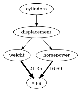
正如我们在这里看到的，重量对mpg方差的影响比马力大得多。

虽然了解直接父节点对我们感兴趣的节点有多大影响提供了一些有价值的见解，但权重和马力可能只是从它们的共同父节点继承信息。为了区分从父节点继承的信息和它们自己的贡献，我们应用了ICC方法：

iccs_mpg = gcm.intrinsic_causal_influence(scm_mpg, target_node='mpg')

Evaluating set functions...: 100%|██████████| 32/32 [00:14<00:00,  2.20it/s]

为了更好地解释结果，我们通过将其归一化到总和上来将方差归因转换为百分比。

def convert_to_percentage(value_dictionary):
    total_absolute_sum = np.sum([abs(v) for v in value_dictionary.values()])
    return {k: abs(v) / total_absolute_sum * 100 for k, v in value_dictionary.items()}

bar_plot(convert_to_percentage(iccs_mpg), ylabel='Variance contribution in %')

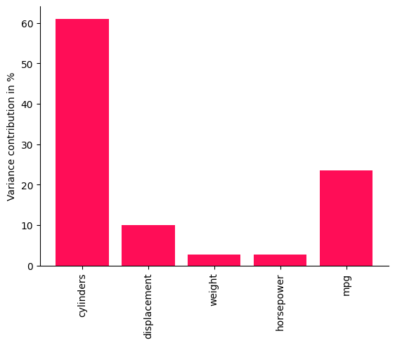
事实证明，气缸数量已经解释了燃油消耗的大部分，而像排量、马力和重量这样的中间节点大多继承了它们父节点的不确定性。这是因为，尽管重量和马力是更直接的mpg预测因素，但它们主要由排量和气缸数量决定。这为潜在的优化提供了一些有用的见解。正如我们在mpg本身的贡献中所看到的，大约1/4的mpg方差仍然无法由上述所有因素解释，这可能部分归因于模型的不准确性。

虽然模型评估显示生成分布与观察分布之间的KL散度存在一些不准确性，但我们看到ICC仍然提供了非平凡的结果，即各节点之间的贡献显著不同，并非所有内容都简单地归因于目标节点本身。

请注意，估计ICC中目标方差的贡献可以被视为一种结合了因果结构的非线性版本的ANOVA。

河流流量的内在影响

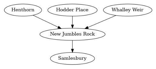
在下一个例子中，我们查看了在英格兰的Henthorn、New Jumbles Rock、Hodder Place、Whalley Weir和Samlesbury五个不同测量站以15分钟频率记录的河流流量（\(m^3/s\)）。这里，更好地理解河流流量的行为有助于规划潜在的缓解措施，以避免溢出。数据取自英国环境食品与农村事务部网站。以下是河流的地图：

新杂石位于三条河流的交汇点，这三条河流分别流经亨索恩、霍德广场和惠利堰，新杂石最终流入萨姆斯伯里。流经某个测量站的水量肯定是上游更远站点观测到的水量的一部分，加上中间流入的小溪和小河的水量。这定义了我们的因果图如下：

river_graph = nx.DiGraph([('Henthorn', 'New Jumbles Rock'),
                          ('Hodder Place', 'New Jumbles Rock'),
                          ('Whalley Weir', 'New Jumbles Rock'),
                          ('New Jumbles Rock', 'Samlesbury')])

plot(river_graph)

在这种情况下，我们对上游河流对Samlesbury河的因果影响感兴趣。与之前的例子类似，我们预计这些节点会受到天气等因素的严重混淆。也就是说，真实的图更可能是这样的：

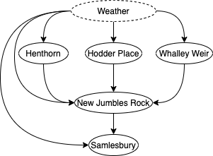
尽管如此，我们仍然期望ICC算法能够提供一些关于Samlesbury河流流量贡献的见解，即使存在隐藏的混杂因素：

river_data = pd.read_csv("river.csv", index_col=False)

scm_river = gcm.StructuralCausalModel(river_graph)
gcm.auto.assign_causal_mechanisms(scm_river, river_data)
gcm.fit(scm_river, river_data)

iccs_river = gcm.intrinsic_causal_influence(scm_river, target_node='Samlesbury')
bar_plot(convert_to_percentage(iccs_river), ylabel='Variance contribution in %')

Fitting causal mechanism of node Samlesbury: 100%|██████████| 5/5 [00:00<00:00, 185.12it/s]
Evaluating set functions...: 100%|██████████| 32/32 [00:00<00:00, 297.94it/s]

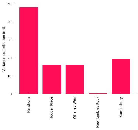
有趣的是，尽管New Jumbles Rock对Samlesbury的内在贡献很小，但对New Jumbles Rock的干预效果肯定会有很大的影响。这说明ICC并不衡量治疗效果强度意义上的影响，并在此指出New Jumbles Rock只是将流量传递到Samlesbury。Samlesbury本身的贡献代表了未被捕捉到的（隐藏）因素。尽管我们可以预期节点会受到天气的严重干扰，但分析仍然提供了一些有趣的见解，这些见解只有通过仔细区分从父节点继承的影响和节点新添加的“信息”才能获得。