使用工具变量方法进行估计的简单示例

%load_ext autoreload
%autoreload 2

import numpy as np
import pandas as pd
import patsy as ps

from statsmodels.sandbox.regression.gmm import IV2SLS
import os, sys
from dowhy import CausalModel

加载数据集

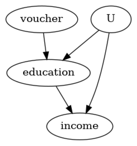
我们创建了一个虚构的数据集，目的是估计教育对个人未来收入的影响。个人的ability是一个混杂因素，而获得education_voucher是工具变量。

n_points = 1000
education_abilty = 1
education_voucher = 2
income_abilty = 2
income_education = 4


# confounder
ability = np.random.normal(0, 3, size=n_points)

# instrument
voucher = np.random.normal(2, 1, size=n_points)

# treatment
education = np.random.normal(5, 1, size=n_points) + education_abilty * ability +\
            education_voucher * voucher

# outcome
income = np.random.normal(10, 3, size=n_points) +\
         income_abilty * ability + income_education * education

# build dataset (exclude confounder `ability` which we assume to be unobserved)
data = np.stack([education, income, voucher]).T
df = pd.DataFrame(data, columns = ['education', 'income', 'voucher'])

使用DoWhy估计教育对未来收入的因果效应

我们遵循以下四个步骤：1）使用因果图对问题进行建模，

2. 识别是否可以从观察到的变量中估计因果效应，

3. 估计效果，并且

4. 检查估计的稳健性。

#Step 1: Model
model=CausalModel(
        data = df,
        treatment='education',
        outcome='income',
        common_causes=['U'],
        instruments=['voucher']
        )
model.view_model()
from IPython.display import Image, display
display(Image(filename="causal_model.png"))

/__w/dowhy/dowhy/dowhy/causal_model.py:583: UserWarning: 1 variables are assumed unobserved because they are not in the dataset. Configure the logging level to `logging.WARNING` or higher for additional details.
  warnings.warn(

# Step 2: Identify
identified_estimand = model.identify_effect(proceed_when_unidentifiable=True)
print(identified_estimand)

Estimand type: EstimandType.NONPARAMETRIC_ATE

### Estimand : 1
Estimand name: backdoor
No such variable(s) found!

### Estimand : 2
Estimand name: iv
Estimand expression:
 ⎡                                            -1⎤
 ⎢    d              ⎛    d                  ⎞  ⎥
E⎢──────────(income)⋅⎜──────────([education])⎟  ⎥
 ⎣d[voucher]         ⎝d[voucher]             ⎠  ⎦
Estimand assumption 1, As-if-random: If U→→income then ¬(U →→{voucher})
Estimand assumption 2, Exclusion: If we remove {voucher}→{education}, then ¬({voucher}→income)

### Estimand : 3
Estimand name: frontdoor
No such variable(s) found!

# Step 3: Estimate
#Choose the second estimand: using IV
estimate = model.estimate_effect(identified_estimand,
        method_name="iv.instrumental_variable", test_significance=True)

print(estimate)

*** Causal Estimate ***

## Identified estimand
Estimand type: EstimandType.NONPARAMETRIC_ATE

### Estimand : 1
Estimand name: iv
Estimand expression:
 ⎡                                            -1⎤
 ⎢    d              ⎛    d                  ⎞  ⎥
E⎢──────────(income)⋅⎜──────────([education])⎟  ⎥
 ⎣d[voucher]         ⎝d[voucher]             ⎠  ⎦
Estimand assumption 1, As-if-random: If U→→income then ¬(U →→{voucher})
Estimand assumption 2, Exclusion: If we remove {voucher}→{education}, then ¬({voucher}→income)

## Realized estimand
Realized estimand: Wald Estimator
Realized estimand type: EstimandType.NONPARAMETRIC_ATE
Estimand expression:
  ⎡   d            ⎤
 E⎢────────(income)⎥
  ⎣dvoucher        ⎦
──────────────────────
 ⎡   d               ⎤
E⎢────────(education)⎥
 ⎣dvoucher           ⎦
Estimand assumption 1, As-if-random: If U→→income then ¬(U →→{voucher})
Estimand assumption 2, Exclusion: If we remove {voucher}→{education}, then ¬({voucher}→income)
Estimand assumption 3, treatment_effect_homogeneity: Each unit's treatment ['education'] is affected in the same way by common causes of ['education'] and ['income']
Estimand assumption 4, outcome_effect_homogeneity: Each unit's outcome ['income'] is affected in the same way by common causes of ['education'] and ['income']

Target units: ate

## Estimate
Mean value: 4.0206040845835105
p-value: [0, 0.001]

我们有一个估计，表明将education增加一个单位会使income增加4个点。

接下来，我们使用安慰剂反驳测试来检查估计的稳健性。在这个测试中，治疗被一个独立的随机变量所取代（同时保持与工具的关联），因此真实的因果效应应该为零。我们检查我们的估计器是否也提供了零的正确答案。

# Step 4: Refute
ref = model.refute_estimate(identified_estimand, estimate, method_name="placebo_treatment_refuter", placebo_type="permute") # only permute placebo_type works with IV estimate
print(ref)

Refute: Use a Placebo Treatment
Estimated effect:4.0206040845835105
New effect:0.07846773265599782
p value:0.72

反驳使我们有信心估计没有捕捉到数据中的任何噪声。

由于这是模拟数据，我们也知道真实的因果效应是 4（参见上面数据生成过程的 income_education 参数）

最后，我们通过另一种方法展示相同的估计，以验证来自DoWhy的结果。

income_vec, endog = ps.dmatrices("income ~ education", data=df)
exog = ps.dmatrix("voucher", data=df)

m = IV2SLS(income_vec, endog, exog).fit()
m.summary()

IV2SLS Regression Results

因变量:	income	R平方:	0.892
模型:	IV2SLS	调整后的R平方:	0.892
方法:	两阶段	F统计量:	1528.
	最小二乘法	Prob (F统计量):	1.93e-203
日期:	2024年11月24日，星期日
时间:	18:03:48
观测数量：	1000
自由度残差:	998
自由度模型:	1

	系数	标准误差	t值	P>|t|	[0.025	0.975]
截距	10.0485	0.957	10.504	0.000	8.171	11.926
教育	4.0206	0.103	39.086	0.000	3.819	4.222

综合统计量:	1.426	杜宾-沃森统计量:	1.933
概率(Omnibus):	0.490	Jarque-Bera (JB):	1.446
偏度:	-0.092	JB概率:	0.485
峰度:	2.966	条件数	26.7