非参数因果估计的敏感性分析#
敏感性分析帮助我们研究当无未观察到的混杂假设被违反时,估计效果的稳健性。也就是说,由于省略了一个(未观察到的)混杂因素,我们的估计有多少偏差?这被称为遗漏变量偏差(OVB),它为我们提供了一个衡量标准,即包含一个被遗漏的共同原因(混杂因素)会如何改变估计效果。
本笔记本展示了如何估计一般非参数因果估计器的OVB。为了获得直观理解,我们建议先阅读一个介绍性笔记本,该笔记本描述了如何为线性估计器估计OVB:线性估计器的敏感性分析。回顾一下,在那个笔记本中,我们看到了OVB如何依赖于线性部分R^2值,并利用这一见解根据混杂因素与结果和治疗的相对强度计算调整后的估计值。我们现在使用非参数部分R^2和Reisz表示器来推广这一技术。
本笔记本基于Chernozhukov等人,长话短说:因果机器学习中的遗漏变量偏差。https://arxiv.org/abs/2112.13398。
I. 部分线性模型的敏感性分析#
我们首先分析当真实的数据生成过程(DGP)已知为部分线性时,因果估计的敏感性。也就是说,结果可以加性地分解为处理的线性函数和混杂因素的非线性函数。我们用\(T\)表示处理,用\(Y\)表示结果,用\(W\)表示观察到的混杂因素,用\(U\)表示未观察到的混杂因素。
然而,我们无法估计上述方程,因为混杂因素 \(U\) 是未观察到的。因此,在实践中,因果估计器使用以下“简化”方程,
敏感性分析的目标是回答\(\theta_s\)与真实的\(\theta\)有多远。Chernozhukov等人表明,给定一个称为Reisz函数的特殊函数\(\alpha\),遗漏变量偏差\(|\theta - \theta_s|\)被\(\sqrt{E[g-g_s]^2E[\alpha-\alpha_s]^2}\)所限制。对于部分线性模型,\(\alpha\)和“短”\(\alpha_s\)被定义为,
这个界限可以用未观察到的混杂因素\(U\)与处理和结果的部分 R^2 来表示,条件是观察到的混杂因素\(W\)。回想一下,\(U\) 相对于某个目标\(Z\)的 R^2 定义为预测\(E[Z|U]\)的方差与\(Z\)的方差的比值,\(R^2_{Z\sim U}=\frac{\operatorname{Var}(E[Z|U])}{\operatorname{Var}(Y)}\)。我们可以将部分 R^2 定义为一个扩展,它衡量了在某些变量\(W\)条件下的额外解释能力。
界限由以下公式给出,
其中,
\(S^2\) 可以从数据中估计。其他两个参数需要手动指定:它们传达了未观察到的混杂因素 \(U\) 对处理和结果的强度。下面我们展示了如何通过为 \(\eta^2_{Y \sim U | T, W}\) 和 \(\eta^2_{T\sim U | W}\) 指定一系列合理值来创建敏感性等高线图。我们还展示了如何将这些值作为由于任何观察到的协变量子集的最大部分 R^2 的一部分进行基准测试和设置。
创建一个具有未观察到的混杂因素的数据集#
[1]:
%load_ext autoreload
%autoreload 2
[2]:
# Required libraries
import re
import numpy as np
import dowhy
from dowhy import CausalModel
import dowhy.datasets
from dowhy.utils.regression import create_polynomial_function
我们创建了一个数据集,其中治疗和结果之间存在线性关系,遵循部分线性数据生成过程。\(\beta\) 是真实的因果效应。
[3]:
np.random.seed(101)
data = dowhy.datasets.partially_linear_dataset(beta = 10,
                                               num_common_causes = 7,
                                               num_unobserved_common_causes=1,
                                               strength_unobserved_confounding=10,
                                               num_samples = 1000,
                                               num_treatments = 1,
                                               stddev_treatment_noise = 10,
                                               stddev_outcome_noise = 5
                                                )
display(data)
{'df':            W0        W1        W2        W3        W4        W5        W6  \
 0    0.345542  0.696984 -0.708658 -1.997165 -0.709139  0.165913 -0.554212
 1   -0.075270  1.652779 -0.259591  0.282963 -0.764418  0.032002 -0.360908
 2   -0.240272 -0.174564 -0.934469 -0.451650  1.959730  1.201015  0.471282
 3    0.119874 -0.256127  0.318636 -0.223625  0.233940  1.549934 -0.763879
 4    0.179436  1.410457 -0.635170 -1.263762  1.289872 -0.528325  0.122878
 ..        ...       ...       ...       ...       ...       ...       ...
 995  1.131240  0.084704 -1.837648 -0.250193 -0.774702 -0.466984 -0.979246
 996 -0.581574  0.167608 -1.914603 -0.653232  2.027677  0.513934 -1.188357
 997  0.009781  2.095094 -1.417172 -0.118229  1.953746  0.357782 -0.129897
 998 -0.310415  0.410795 -0.205454 -0.818042  0.747265  1.235053  0.627017
 999 -0.015367 -0.026768 -0.390476 -0.064762 -0.095389  0.911950  0.329420

         v0          y
 0     True   8.391102
 1     True  21.853491
 2    False   1.247109
 3     True  13.881250
 4     True  13.929866
 ..     ...        ...
 995   True  14.289693
 996  False   6.831359
 997   True  10.695485
 998  False  -8.849379
 999   True  13.994482

 [1000 rows x 9 columns],
 'treatment_name': ['v0'],
 'outcome_name': 'y',
 'common_causes_names': ['W0', 'W1', 'W2', 'W3', 'W4', 'W5', 'W6'],
 'dot_graph': 'digraph {v0->y;W0-> v0; W1-> v0; W2-> v0; W3-> v0; W4-> v0; W5-> v0; W6-> v0;W0-> y; W1-> y; W2-> y; W3-> y; W4-> y; W5-> y; W6-> y;}',
 'gml_graph': 'graph[directed 1node[ id "y" label "y"]node[ id "W0" label "W0"] node[ id "W1" label "W1"] node[ id "W2" label "W2"] node[ id "W3" label "W3"] node[ id "W4" label "W4"] node[ id "W5" label "W5"] node[ id "W6" label "W6"]node[ id "v0" label "v0"]edge[source "v0" target "y"]edge[ source "W0" target "v0"] edge[ source "W1" target "v0"] edge[ source "W2" target "v0"] edge[ source "W3" target "v0"] edge[ source "W4" target "v0"] edge[ source "W5" target "v0"] edge[ source "W6" target "v0"]edge[ source "W0" target "y"] edge[ source "W1" target "y"] edge[ source "W2" target "y"] edge[ source "W3" target "y"] edge[ source "W4" target "y"] edge[ source "W5" target "y"] edge[ source "W6" target "y"]]',
 'ate': 10.085246711266985}
这个数据生成过程的真实ATE是,
[4]:
data["ate"]
[4]:
为了模拟未观察到的混杂因素,我们从数据集中移除一个常见原因。
[5]:
# Observed data
dropped_cols=["W0"]
user_data = data["df"].drop(dropped_cols, axis = 1)
# assumed graph
user_graph = data["gml_graph"]
for col in dropped_cols:
    user_graph = user_graph.replace('node[ id "{0}" label "{0}"]'.format(col), '')
    user_graph = re.sub('edge\[ source "{}" target "[vy][0]*"\]'.format(col), "", user_graph)
user_data
[5]:
| W1 | W2 | W3 | W4 | W5 | W6 | v0 | y | |
|---|---|---|---|---|---|---|---|---|
| 0 | 0.696984 | -0.708658 | -1.997165 | -0.709139 | 0.165913 | -0.554212 | True | 8.391102 |
| 1 | 1.652779 | -0.259591 | 0.282963 | -0.764418 | 0.032002 | -0.360908 | True | 21.853491 |
| 2 | -0.174564 | -0.934469 | -0.451650 | 1.959730 | 1.201015 | 0.471282 | False | 1.247109 |
| 3 | -0.256127 | 0.318636 | -0.223625 | 0.233940 | 1.549934 | -0.763879 | True | 13.881250 |
| 4 | 1.410457 | -0.635170 | -1.263762 | 1.289872 | -0.528325 | 0.122878 | True | 13.929866 |
| ... | ... | ... | ... | ... | ... | ... | ... | ... |
| 995 | 0.084704 | -1.837648 | -0.250193 | -0.774702 | -0.466984 | -0.979246 | True | 14.289693 |
| 996 | 0.167608 | -1.914603 | -0.653232 | 2.027677 | 0.513934 | -1.188357 | False | 6.831359 |
| 997 | 2.095094 | -1.417172 | -0.118229 | 1.953746 | 0.357782 | -0.129897 | True | 10.695485 |
| 998 | 0.410795 | -0.205454 | -0.818042 | 0.747265 | 1.235053 | 0.627017 | False | -8.849379 |
| 999 | -0.026768 | -0.390476 | -0.064762 | -0.095389 | 0.911950 | 0.329420 | True | 13.994482 |
1000 行 × 8 列
使用模型、识别、估计步骤获取因果估计#
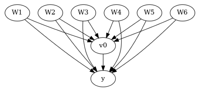
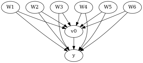
使用“观察到的”数据和因果图创建一个因果模型。
[6]:
model = CausalModel(
            data=user_data,
            treatment=data["treatment_name"],
            outcome=data["outcome_name"],
            graph=user_graph,
            test_significance=None,
        )
model.view_model()
from IPython.display import Image, display
display(Image(filename="causal_model.png"))
[7]:
# Identify effect
identified_estimand = model.identify_effect(proceed_when_unidentifiable=True)
print(identified_estimand)
Estimand type: EstimandType.NONPARAMETRIC_ATE

### Estimand : 1
Estimand name: backdoor
Estimand expression:
  d
─────(E[y|W1,W6,W3,W4,W5,W2])
d[v₀]
Estimand assumption 1, Unconfoundedness: If U→{v0} and U→y then P(y|v0,W1,W6,W3,W4,W5,W2,U) = P(y|v0,W1,W6,W3,W4,W5,W2)

### Estimand : 2
Estimand name: iv
No such variable(s) found!

### Estimand : 3
Estimand name: frontdoor
No such variable(s) found!
[8]:
# Estimate effect
import econml
from sklearn.ensemble import GradientBoostingRegressor
linear_dml_estimate = model.estimate_effect(identified_estimand,
                                    method_name="backdoor.econml.dml.dml.LinearDML",
                                    method_params={
                                        'init_params': {'model_y':GradientBoostingRegressor(),
                                                        'model_t': GradientBoostingRegressor(),
                                                        'linear_first_stages': False
                                                       },
                                        'fit_params': {'cache_values': True,}
                                     })
print(linear_dml_estimate)
A column-vector y was passed when a 1d array was expected. Please change the shape of y to (n_samples, ), for example using ravel().
A column-vector y was passed when a 1d array was expected. Please change the shape of y to (n_samples, ), for example using ravel().
*** Causal Estimate ***

## Identified estimand
Estimand type: EstimandType.NONPARAMETRIC_ATE

### Estimand : 1
Estimand name: backdoor
Estimand expression:
  d
─────(E[y|W1,W6,W3,W4,W5,W2])
d[v₀]
Estimand assumption 1, Unconfoundedness: If U→{v0} and U→y then P(y|v0,W1,W6,W3,W4,W5,W2,U) = P(y|v0,W1,W6,W3,W4,W5,W2)

## Realized estimand
b: y~v0+W1+W6+W3+W4+W5+W2 |
Target units: ate

## Estimate
Mean value: 11.709254833402818
Effect estimates: [[11.70925483]]
使用Refute步骤进行敏感性分析#
在估计之后,我们需要检查我们的估计对于未观察到的混杂因素的可能性有多稳健。我们对LinearDML估计器进行敏感性分析,假设其对数据生成过程的假设成立:\(Y\)的真实函数是部分线性的。为了提高计算效率,我们在fit_params中设置cache_values = True以缓存第一阶段估计的结果。
使用的参数:
method_name: 反驳方法名称
simulation_method: “non-parametric-partial-R2” 用于非参数敏感性分析。请注意,如果使用 LinearDML 估计器进行估计,则会自动选择部分线性敏感性分析。
partial_r2_confounder_treatment: \(\eta^2_{T\sim U | W}\), 在所有观察到的混杂因素条件下,未观察到的混杂因素与治疗的部分R2。
partial_r2_confounder_outcome: \(\eta^2_{Y \sim U | T, W}\), 未观察到的混杂变量与结果的部分R2,条件是处理变量和所有观察到的混杂变量。
[9]:
refute = model.refute_estimate(identified_estimand, linear_dml_estimate ,
                               method_name = "add_unobserved_common_cause",
                               simulation_method = "non-parametric-partial-R2",
                               partial_r2_confounder_treatment = np.arange(0, 0.8, 0.1),
                               partial_r2_confounder_outcome = np.arange(0, 0.8, 0.1)
                              )
print(refute)
Sensitivity Analysis to Unobserved Confounding using partial R^2 parameterization

Original Effect Estimate : 11.709254833402818
Robustness Value : 0.45

Robustness Value (alpha=0.05) : 0.41000000000000003

Interpretation of results :
Any confounder explaining less than 45.0% percent of the residual variance of both the treatment and the outcome would not be strong enough to explain away the observed effect i.e bring down the estimate to 0

For a significance level of 5.0%, any confounder explaining more than 41.0% percent of the residual variance of both the treatment and the outcome would be strong enough to make the estimated effect not 'statistically significant'
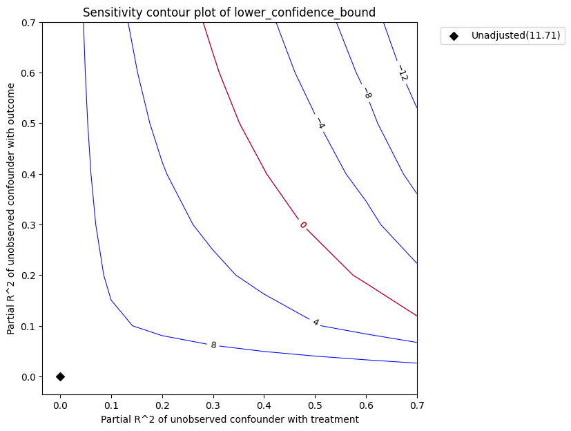
图的解释。 在上图中,x轴显示了未观察到的混杂因素与治疗的假设部分R2值。y轴显示了未观察到的混杂因素与结果的假设部分R2值。在
等高线代表的是如果未观察到的混杂因素被包含在估计模型中,将获得的效应的调整后下置信界估计。红色等高线是调整后效应变为零的临界阈值。因此,具有这种强度或更强的混杂因素足以逆转估计效应的符号并使估计的结论无效。这一概念可以通过输出稳健性值来量化。
[10]:
refute.RV
[10]:
稳健性值衡量了\(\eta^2_{T\sim U | W}\)和\(\eta^2_{Y \sim U | T, W}\)的最小等强度,使得平均处理效应的界限将包括零。它可以在0到1之间。稳健性值为0.45意味着\(\eta^2_{T\sim U | W}\)和\(\eta^2_{Y \sim U | T, W}\)值小于0.4的混杂因素不足以将估计值降至零。一般来说,较低的稳健性值意味着结果可能会因存在较弱的混杂因素而改变,而接近1的稳健性值意味着处理效应甚至可以处理可能解释治疗和结果所有剩余变异的强混杂因素。
基准测试。 然而,通常情况下,提供一个合理的部分R2值范围是困难的。相反,我们可以将未观察到的混杂因素的部分R2推断为任何观察到的混杂因素子集的部分R2的倍数。因此,现在我们只需要将未观察到的混杂效应指定为观察到的混杂效应的倍数/分数。这个过程被称为基准测试。
用于基准测试的相关参数是:- benchmark_common_causes:用于限制未观察到的混杂因素强度的观察到的混杂因素名称 - effect_fraction_on_treatment:未观察到的混杂因素与治疗之间的关联强度与基准混杂因素相比 - effect_fraction_on_outcome:未观察到的混杂因素与结果之间的关联强度与基准混杂因素相比
[11]:
refute_bm = model.refute_estimate(identified_estimand, linear_dml_estimate ,
                               method_name = "add_unobserved_common_cause",
                               simulation_method = "non-parametric-partial-R2",
                               benchmark_common_causes = ["W1"],
                               effect_fraction_on_treatment = 0.2,
                               effect_fraction_on_outcome = 0.2
                              )
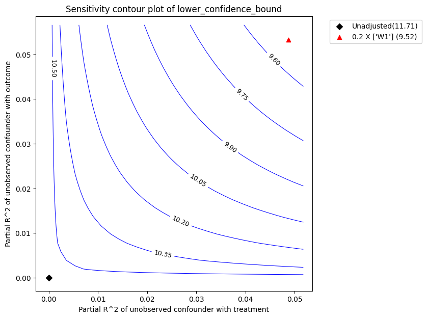
红色三角形显示了所选基准观测协变量与处理和结果的估计部分R^2。在上述调用中,我们选择了W1作为基准协变量。假设未观察到的混杂因素对处理和结果的影响不能比观察到的基准协变量(W1)更强,上图显示在考虑未观察到的混杂因素后,平均估计效应将减少,但仍显著高于零。
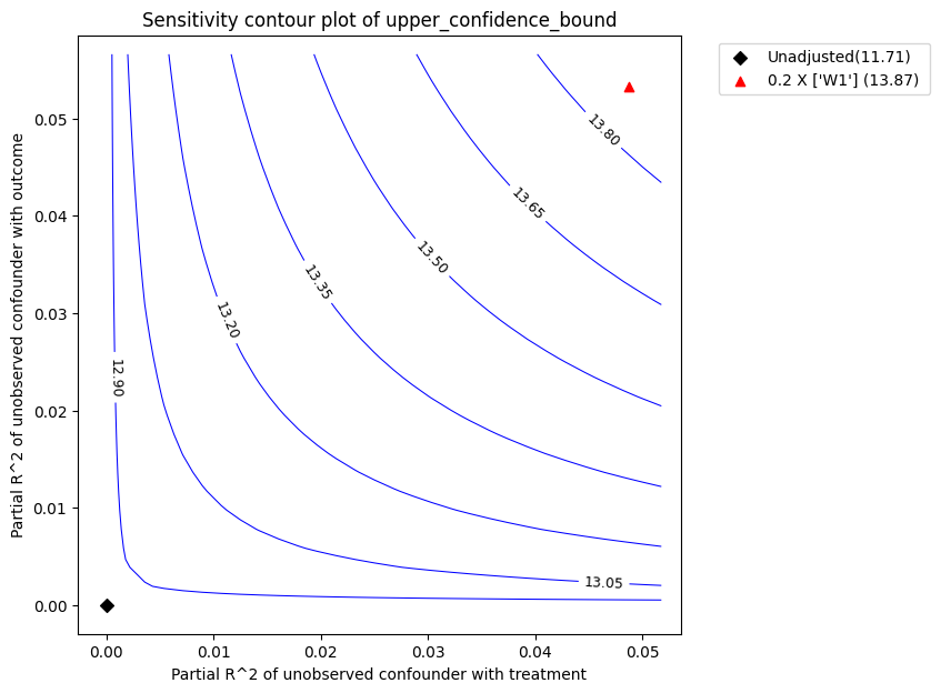
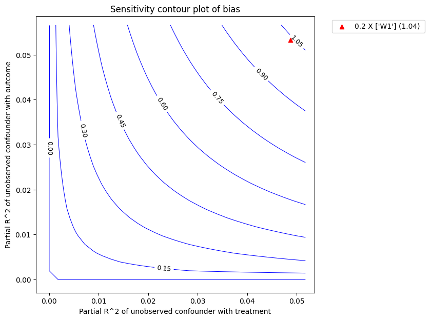
绘图类型。默认的plot_type是显示在显著性水平下的lower_confidence_bound。plot_type的其他可能值包括:* upper_confidence_bound:在预期未观察到的混杂因素会降低估计值的情况下优先使用。* lower_ate_bound:不考虑显著性水平的无混杂平均处理效应的下限(点)估计值 * upper_ate_bound:不考虑显著性水平的无混杂平均处理效应的上限(点)估计值 * bias:获得的估计值与真实估计值相比的偏差
[12]:
refute_bm.plot(plot_type = "upper_confidence_bound")
refute_bm.plot(plot_type = "bias")
我们还可以将基准测试结果作为数据框访问。
[13]:
refute_bm.results
[13]:
| r2tu_w | r2yu_tw | 短期估计 | 偏差 | 下限_ate_bound | 上限_ate_bound | 下限_confidence_bound | 上限_confidence_bound | |
|---|---|---|---|---|---|---|---|---|
| 0 | 0.0487 | 0.053207 | 11.709255 | 1.038683 | 10.670572 | 12.747937 | 9.522549 | 13.868991 |
II. 一般非参数模型的敏感性分析#
我们现在在不假设真实数据生成过程的情况下进行敏感性分析。敏感性仍然取决于未观察到的混杂因素与结果的部分R2,\(\eta^2_{Y \sim U | T, W}\),以及一个类似的混杂因素-治疗关系参数。然而,边界的计算更为复杂,需要估计一个称为reisz函数的特殊函数。详情请参考Chernozhukov等人的研究。
[14]:
# Estimate effect using a non-parametric estimator
from sklearn.ensemble import GradientBoostingRegressor
estimate_npar = model.estimate_effect(identified_estimand,
                                    method_name="backdoor.econml.dml.KernelDML",
                                    method_params={
                                        'init_params': {'model_y':GradientBoostingRegressor(),
                                                        'model_t': GradientBoostingRegressor(),                                                       },
                                        'fit_params': {},
                                     })
print(estimate_npar)
A column-vector y was passed when a 1d array was expected. Please change the shape of y to (n_samples, ), for example using ravel().
A column-vector y was passed when a 1d array was expected. Please change the shape of y to (n_samples, ), for example using ravel().
*** Causal Estimate ***

## Identified estimand
Estimand type: EstimandType.NONPARAMETRIC_ATE

### Estimand : 1
Estimand name: backdoor
Estimand expression:
  d
─────(E[y|W1,W6,W3,W4,W5,W2])
d[v₀]
Estimand assumption 1, Unconfoundedness: If U→{v0} and U→y then P(y|v0,W1,W6,W3,W4,W5,W2,U) = P(y|v0,W1,W6,W3,W4,W5,W2)

## Realized estimand
b: y~v0+W1+W6+W3+W4+W5+W2 |
Target units: ate

## Estimate
Mean value: 11.831292187241948
Effect estimates: [[11.83129219]]
为了进行敏感性分析,我们现在使用相同的non-parametric--partial-R2方法,然而部分R2的估计将基于reisz表示器。我们使用plugin_reisz=True来指定我们将使用插件reisz函数估计器(这更快且适用于二元处理)。否则,我们可以将其设置为False以使用损失函数来估计reisz函数。
[15]:
refute_npar = model.refute_estimate(identified_estimand, estimate_npar,
                               method_name = "add_unobserved_common_cause",
                               simulation_method = "non-parametric-partial-R2",
                               benchmark_common_causes = ["W1"],
                               effect_fraction_on_treatment = 0.2,
                               effect_fraction_on_outcome = 0.2,
                               plugin_reisz=True
                              )
print(refute_npar)
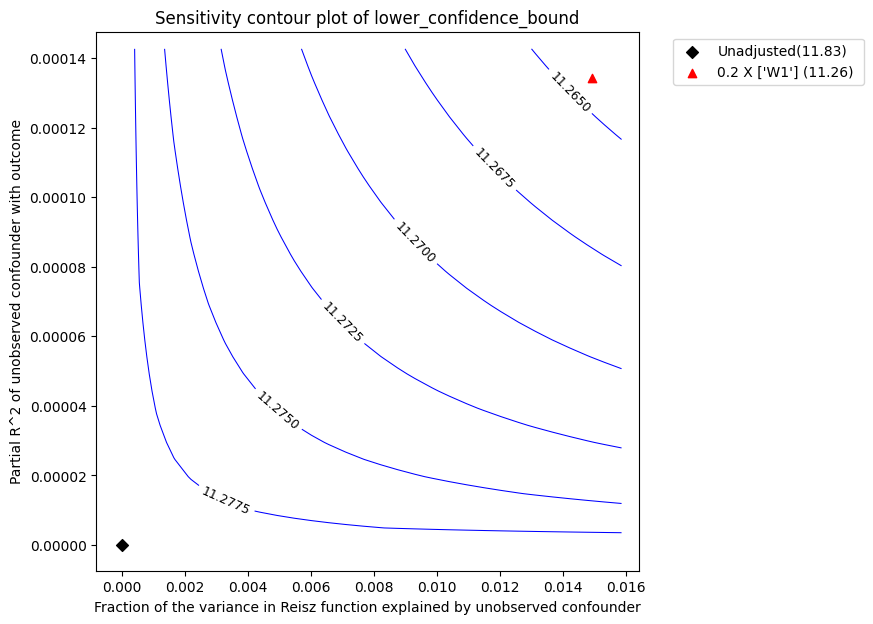
Sensitivity Analysis to Unobserved Confounding using partial R^2 parameterization

Original Effect Estimate : 11.831292187241948
Robustness Value : 0.66

Robustness Value (alpha=0.05) : 0.64

Interpretation of results :
Any confounder explaining less than 66.0% percent of the residual variance of both the treatment and the outcome would not be strong enough to explain away the observed effect i.e bring down the estimate to 0

For a significance level of 5.0%, any confounder explaining more than 64.0% percent of the residual variance of both the treatment and the outcome would be strong enough to make the estimated effect not 'statistically significant'
该图表的解释与之前相同。我们获得的稳健性值为0.66,而LinearDML估计器的稳健性值为0.45。
请注意,尽管LinearDML和KernelDML的点估计相似,但稳健性值发生了变化。这是因为我们对真实数据生成过程做出了不同的假设。