回归模型的敏感性分析#
Sensitivity analysis helps us examine how sensitive a result is against the possibility of unobserved confounding. Two methods are implemented: 1. Cinelli & Hazlett’s robustness value - This method only supports linear regression estimator. - The partial R^2 of treatment with outcome shows how strongly confounders explaining all the residual outcome variation would have to be associated with the treatment to eliminate the estimated effect. - The robustness value measures the minimum strength of association unobserved confounding should have with both treatment and outcome in order to change the conclusions. - Robustness value close to 1 means the treatment effect can handle strong confounders explaining almost all residual variation of the treatment and the outcome. - Robustness value close to 0 means that even very weak confounders can also change the results. - Benchmarking examines the sensitivity of causal inferences to plausible strengths of the omitted confounders. - This method is based on https://carloscinelli.com/files/Cinelli%20and%20Hazlett%20(2020)%20-%20Making%20Sense%20of%20Sensitivity.pdf 2. Ding & VanderWeele’s E-Value - This method supports linear and logistic regression. - The E-value is the minimum strength of association on the risk ratio scale that an unmeasured confounder would need to have with both the treatment and the outcome, conditional on the measured covariates, to fully explain away a specific treatment-outcome association. - The minimum E-value is 1, which means that no unmeasured confounding is needed to explain away the observed association (i.e. the confidence interval crosses the null). - Higher E-values mean that stronger unmeasured confounding is needed to explain away the observed association. There is no maximum E-value. - McGowan & Greevy Jr’s benchmarks the E-value against the measured confounders.
步骤1:加载所需的包#
[1]:
import os, sys
sys.path.append(os.path.abspath("../../../"))
import dowhy
from dowhy import CausalModel
import pandas as pd
import numpy as np
import dowhy.datasets

# Config dict to set the logging level
import logging.config
DEFAULT_LOGGING = {
    'version': 1,
    'disable_existing_loggers': False,
    'loggers': {
        '': {
            'level': 'ERROR',
        },
    }
}

logging.config.dictConfig(DEFAULT_LOGGING)
# Disabling warnings output
import warnings
from sklearn.exceptions import DataConversionWarning
#warnings.filterwarnings(action='ignore', category=DataConversionWarning)
步骤2:加载数据集#
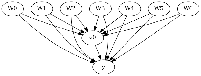
我们创建了一个数据集,其中常见原因与治疗之间以及常见原因与结果之间存在线性关系。Beta 是真实的因果效应。
[2]:
np.random.seed(100)
data = dowhy.datasets.linear_dataset( beta = 10,
                                      num_common_causes = 7,
                                      num_samples = 500,
                                      num_treatments = 1,
                                     stddev_treatment_noise =10,
                                     stddev_outcome_noise = 5
                                    )
[3]:
model = CausalModel(
data=data["df"],
treatment=data["treatment_name"],
outcome=data["outcome_name"],
graph=data["gml_graph"],
test_significance=None,
)
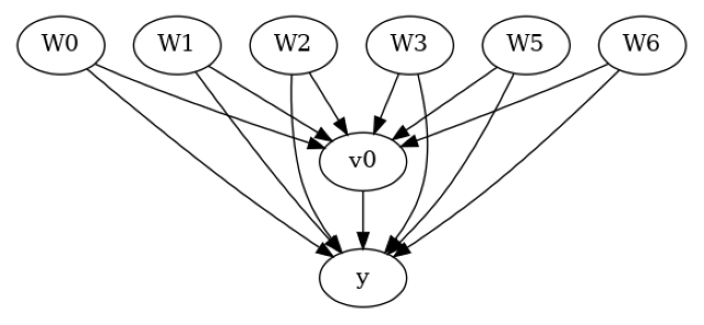
model.view_model()
from IPython.display import Image, display
display(Image(filename="causal_model.png"))
data['df'].head()


[3]:
| W0 | W1 | W2 | W3 | W4 | W5 | W6 | v0 | y | |
|---|---|---|---|---|---|---|---|---|---|
| 0 | -0.145062 | -0.235286 | 0.784843 | 0.869131 | -1.567724 | -1.290234 | 0.116096 | True | 1.386517 |
| 1 | -0.228109 | -0.020264 | -0.589792 | 0.188139 | -2.649265 | -1.764439 | -0.167236 | False | -16.159402 |
| 2 | 0.868298 | -1.097642 | -0.109792 | 0.487635 | -1.861375 | -0.527930 | -0.066542 | False | -0.702560 |
| 3 | -0.017115 | 1.123918 | 0.346060 | 1.845425 | 0.848049 | 0.778865 | 0.596496 | True | 27.714465 |
| 4 | -0.757347 | -1.426205 | -0.457063 | 1.528053 | -2.681410 | 0.394312 | -0.687839 | False | -20.082633 |
步骤3:创建因果模型#
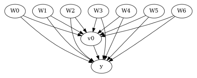
移除一个常见原因以模拟未观察到的混杂因素
[4]:
data["df"] = data["df"].drop("W4", axis = 1)
graph_str = 'graph[directed 1node[ id "y" label "y"]node[ id "W0" label "W0"] node[ id "W1" label "W1"] node[ id "W2" label "W2"] node[ id "W3" label "W3"] node[ id "W5" label "W5"] node[ id "W6" label "W6"]node[ id "v0" label "v0"]edge[source "v0" target "y"]edge[ source "W0" target "v0"] edge[ source "W1" target "v0"] edge[ source "W2" target "v0"] edge[ source "W3" target "v0"] edge[ source "W5" target "v0"] edge[ source "W6" target "v0"]edge[ source "W0" target "y"] edge[ source "W1" target "y"] edge[ source "W2" target "y"] edge[ source "W3" target "y"] edge[ source "W5" target "y"] edge[ source "W6" target "y"]]'
model = CausalModel(
data=data["df"],
treatment=data["treatment_name"],
outcome=data["outcome_name"],
graph=graph_str,
test_significance=None,
)
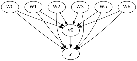
model.view_model()
from IPython.display import Image, display
display(Image(filename="causal_model.png"))
data['df'].head()
[4]:
| W0 | W1 | W2 | W3 | W5 | W6 | v0 | y | |
|---|---|---|---|---|---|---|---|---|
| 0 | -0.145062 | -0.235286 | 0.784843 | 0.869131 | -1.290234 | 0.116096 | True | 1.386517 |
| 1 | -0.228109 | -0.020264 | -0.589792 | 0.188139 | -1.764439 | -0.167236 | False | -16.159402 |
| 2 | 0.868298 | -1.097642 | -0.109792 | 0.487635 | -0.527930 | -0.066542 | False | -0.702560 |
| 3 | -0.017115 | 1.123918 | 0.346060 | 1.845425 | 0.778865 | 0.596496 | True | 27.714465 |
| 4 | -0.757347 | -1.426205 | -0.457063 | 1.528053 | 0.394312 | -0.687839 | False | -20.082633 |
步骤4:识别#
[5]:
identified_estimand = model.identify_effect(proceed_when_unidentifiable=True)
print(identified_estimand)
Estimand type: EstimandType.NONPARAMETRIC_ATE

### Estimand : 1
Estimand name: backdoor
Estimand expression:
  d
─────(E[y|W3,W6,W1,W5,W0,W2])
d[v₀]
Estimand assumption 1, Unconfoundedness: If U→{v0} and U→y then P(y|v0,W3,W6,W1,W5,W0,W2,U) = P(y|v0,W3,W6,W1,W5,W0,W2)

### Estimand : 2
Estimand name: iv
No such variable(s) found!

### Estimand : 3
Estimand name: frontdoor
No such variable(s) found!
步骤5:估计#
目前仅支持线性回归估计器用于线性敏感性分析
[6]:
estimate = model.estimate_effect(identified_estimand,method_name="backdoor.linear_regression")
print(estimate)
*** Causal Estimate ***

## Identified estimand
Estimand type: EstimandType.NONPARAMETRIC_ATE

### Estimand : 1
Estimand name: backdoor
Estimand expression:
  d
─────(E[y|W3,W6,W1,W5,W0,W2])
d[v₀]
Estimand assumption 1, Unconfoundedness: If U→{v0} and U→y then P(y|v0,W3,W6,W1,W5,W0,W2,U) = P(y|v0,W3,W6,W1,W5,W0,W2)

## Realized estimand
b: y~v0+W3+W6+W1+W5+W0+W2
Target units: ate

## Estimate
Mean value: 10.697677486880925
步骤6a:反驳和敏感性分析 - 方法1#
identified_estimand: identifiedEstimand 类的一个实例,提供有关因果路径的信息,当处理影响结果时使用 estimate: CausalEstimate 类的一个实例。从原始数据的估计器获得的估计 method_name: 反驳方法名称 simulation_method: “linear-partial-R2” 用于线性敏感性分析 benchmark_common_causes: 用于限制未观察到的混杂因素强度的协变量名称 percent_change_estimate: 这是可以改变结果的处理估计的减少百分比(默认 = 1)如果 percent_change_estimate = 1,稳健性值描述了混杂因素与处理和结果之间的关联强度,以便将估计减少 100%,即将其降至 0。confounder_increases_estimate: confounder_increases_estimate = True 意味着混杂因素增加估计的绝对值,反之亦然。默认是 confounder_increases_estimate = False,即所考虑的混杂因素将估计拉向零 effect_fraction_on_treatment: 未观察到的混杂因素与处理之间的关联强度与基准协变量相比 effect_fraction_on_outcome: 未观察到的混杂因素与结果之间的关联强度与基准协变量相比 null_hypothesis_effect: 零假设下的假设效应(默认 = 0) plot_estimate: 在执行敏感性分析时生成估计的等高线图。(默认 = True)。要覆盖此设置,请设置 plot_estimate = False。
[7]:
refute = model.refute_estimate(identified_estimand, estimate ,
method_name = "add_unobserved_common_cause",
simulation_method = "linear-partial-R2",
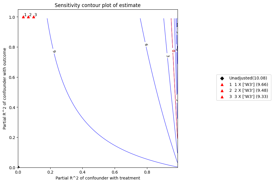
benchmark_common_causes = ["W3"],
effect_fraction_on_treatment = [ 1,2,3]
)
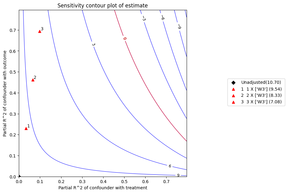
x轴显示了未观察到的混杂因素与治疗之间的假设部分R2值。y轴显示了未观察到的混杂因素与结果之间的假设部分R2值。等高线水平表示当这些假设的部分R2值被包含在完整回归模型中时,未观察到的混杂因素的调整t值或估计值。红线是临界阈值:具有这种强度或更强的混杂因素足以使研究结论无效。
[8]:
refute.stats
[8]:
{'estimate': 10.697677486880925,
 'standard_error': 0.5938735661282949,
 'degree of freedom': 492,
 't_statistic': 18.013392238727626,
 'r2yt_w': 0.3974149837266683,
 'partial_f2': 0.6595168698094567,
 'robustness_value': 0.5467445572181009,
 'robustness_value_alpha': 0.5076289101030926}
[9]:
refute.benchmarking_results
[9]:
| r2tu_w | r2yu_tw | 偏差调整估计 | 偏差调整标准误差 | 偏差调整t值 | 偏差调整置信区间下限 | 偏差调整置信区间上限 | |
|---|---|---|---|---|---|---|---|
| 0 | 0.032677 | 0.230238 | 9.535964 | 0.530308 | 17.981928 | 8.494016 | 10.577912 |
| 1 | 0.065354 | 0.461490 | 8.331381 | 0.451241 | 18.463243 | 7.444783 | 9.217979 |
| 2 | 0.098031 | 0.693855 | 7.080284 | 0.346341 | 20.443123 | 6.399795 | 7.760773 |
plot函数的参数列表#
plot_type: “estimate” 或 “t-value” critical_value: 估计值或t值的特殊参考值,将在图中高亮显示 x_limit: 图的最大x轴值(默认 = 0.8) y_limit: 图的最小y轴值(默认 = 0.8) num_points_per_contour: 计算和绘制每条等高线的点数(默认 = 200) plot_size: 表示图大小的元组(默认 = (7,7)) contours_color: 等高线颜色(默认 = 蓝色) 字符串或数组。如果是数组,线条将按升序绘制特定颜色。 critical_contour_color: 阈值线颜色(默认 = 红色) label_fontsize: 等高线标签的字体大小(默认 = 9) contour_linewidths: 等高线的线宽(默认 = 0.75) contour_linestyles: 等高线的线型(默认 = “solid”) 参见:https://matplotlib.org/3.5.0/gallery/lines_bars_and_markers/linestyles.html contours_label_color: 等高线标签颜色(默认 = 黑色) critical_label_color: 阈值线标签颜色(默认 = 红色) unadjusted_estimate_marker: 图中未调整估计值的标记类型(默认 = ‘D’) 参见:https://matplotlib.org/stable/api/markers_api.html unadjusted_estimate_color: 图中未调整估计值的标记颜色(默认 = “黑色”) adjusted_estimate_marker: 图中偏差调整估计值的标记类型(默认 = ‘^’)adjusted_estimate_color: 图中偏差调整估计值的标记颜色(默认 = “红色”) legend_position: 表示图例位置的元组(默认 = (1.6, 0.6))
[10]:
refute.plot(plot_type = 't-value')
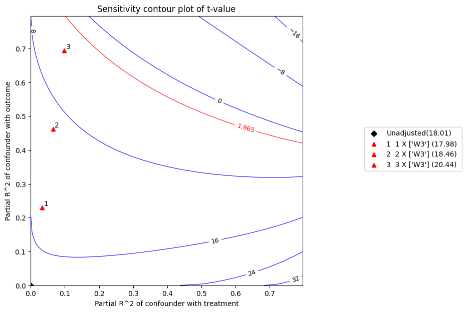
t统计量是系数除以其标准误差。t值越高,拒绝零假设的证据越强。根据上图,在5%的显著性水平下,考虑到上述混杂因素,零效应假设将被拒绝。
[11]:
print(refute)
Sensitivity Analysis to Unobserved Confounding using R^2 paramterization

Unadjusted Estimates of Treatment ['v0'] :
Coefficient Estimate : 10.697677486880925
Degree of Freedom : 492
Standard Error : 0.5938735661282949
t-value : 18.013392238727626
F^2 value : 0.6595168698094567

Sensitivity Statistics :
Partial R2 of treatment with outcome : 0.3974149837266683
Robustness Value : 0.5467445572181009

Interpretation of results :
Any confounder explaining less than 54.67% percent of the residual variance of both the treatment and the outcome would not be strong enough to explain away the observed effect i.e bring down the estimate to 0

For a significance level of 5.0%, any confounder explaining more than 50.76% percent of the residual variance of both the treatment and the outcome would be strong enough to make the estimated effect not 'statistically significant'

If confounders explained 100% of the residual variance of the outcome, they would need to explain at least 39.74% of the residual variance of the treatment to bring down the estimated effect to 0
步骤6b:反驳和敏感性分析 - 方法2#
simulated_method_name: “e-value” 用于 E-value
num_points_per_contour: 每个等高线计算和绘制的点数(默认 = 200)
plot_size: 图表的大小(默认 = (6.4,4.8))
contour_colors: 点估计和置信限轮廓的颜色(默认 = [“blue”, “red])
xy_limit: 绘图的最大x和y值。默认是2倍的E值。(默认 = None)
[12]:
refute = model.refute_estimate(identified_estimand, estimate ,
                               method_name = "add_unobserved_common_cause",
                               simulation_method = "e-value",
                              )
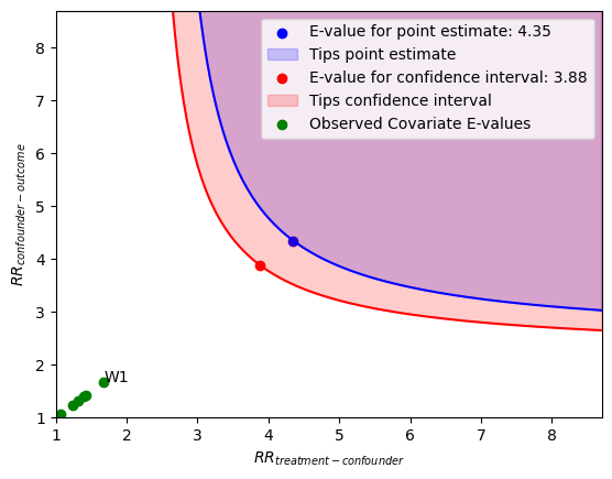
x轴显示了未测量混杂因素在不同治疗水平下的风险比的假设值。y轴显示了混杂因素在不同水平下结果的风险比的假设值。
位于或高于蓝色等高线的点表示这些风险比的组合,这些组合将推翻(即解释掉)点估计。
位于或高于红色等高线的点表示这些风险比的组合,这些组合将翻转(即解释掉)置信区间。
绿色点是观察到的协变量E值。这些值衡量了在删除特定协变量并重新拟合估计器后,置信区间的极限边界在E值尺度上的变化程度。标记了对应于最大观察协变量E值的协变量。
[13]:
refute.stats
[13]:
{'converted_estimate': 2.4574470657354244,
 'converted_lower_ci': 2.2288567270043154,
 'converted_upper_ci': 2.7094815057979966,
 'evalue_estimate': 4.349958364289867,
 'evalue_lower_ci': 3.883832733630416,
 'evalue_upper_ci': None}
[14]:
refute.benchmarking_results
[14]:
| 转换后的估计值 | 转换后的置信区间下限 | 转换后的置信区间上限 | 观察到的协变量E值 | |
|---|---|---|---|---|
| dropped_covariate | ||||
| W1 | 2.992523 | 2.666604 | 3.358276 | 1.681140 |
| W6 | 2.687656 | 2.446341 | 2.952774 | 1.424835 |
| W3 | 2.692807 | 2.422402 | 2.993396 | 1.394043 |
| W0 | 2.599868 | 2.368550 | 2.853776 | 1.320751 |
| W5 | 2.553701 | 2.315245 | 2.816716 | 1.239411 |
| W2 | 2.473648 | 2.217699 | 2.759138 | 1.076142 |
[15]:
print(refute)
Sensitivity Analysis to Unobserved Confounding using the E-value

Unadjusted Estimates of Treatment: v0
Estimate (converted to risk ratio scale): 2.4574470657354244
Lower 95% CI (converted to risk ratio scale): 2.2288567270043154
Upper 95% CI (converted to risk ratio scale): 2.7094815057979966

Sensitivity Statistics:
E-value for point estimate: 4.349958364289867
E-value for lower 95% CI: 3.883832733630416
E-value for upper 95% CI: None
Largest Observed Covariate E-value: 1.6811401167656765 (W1)

Interpretation of results:
Unmeasured confounder(s) would have to be associated with a 4.35-fold increase in the risk of y, and must be 4.35 times more prevalent in v0, to explain away the observed point estimate.
Unmeasured confounder(s) would have to be associated with a 3.88-fold increase in the risk of y, and must be 3.88 times more prevalent in v0, to explain away the observed confidence interval.
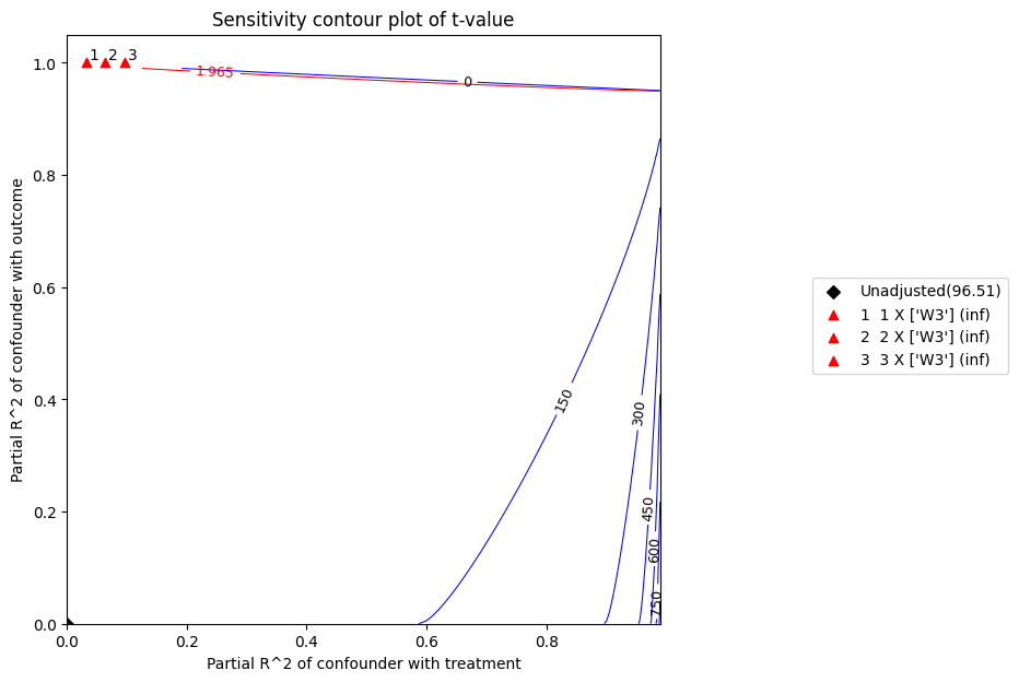
我们现在对相同的数据集进行敏感性分析,但不删除任何变量。我们得到的稳健性值从0.55到0.95,这意味着处理效应可以处理强混杂因素,解释几乎所有的处理和结果的剩余变异。
[16]:
np.random.seed(100)
data = dowhy.datasets.linear_dataset( beta = 10,
                                      num_common_causes = 7,
                                      num_samples = 500,
                                      num_treatments = 1,
                                     stddev_treatment_noise=10,
                                     stddev_outcome_noise = 1
                                    )
[17]:
model = CausalModel(
            data=data["df"],
            treatment=data["treatment_name"],
            outcome=data["outcome_name"],
            graph=data["gml_graph"],
            test_significance=None,
        )
model.view_model()
from IPython.display import Image, display
display(Image(filename="causal_model.png"))
data['df'].head()
[17]:
| W0 | W1 | W2 | W3 | W4 | W5 | W6 | v0 | y | |
|---|---|---|---|---|---|---|---|---|---|
| 0 | -0.145062 | -0.235286 | 0.784843 | 0.869131 | -1.567724 | -1.290234 | 0.116096 | True | 6.311809 |
| 1 | -0.228109 | -0.020264 | -0.589792 | 0.188139 | -2.649265 | -1.764439 | -0.167236 | False | -12.274406 |
| 2 | 0.868298 | -1.097642 | -0.109792 | 0.487635 | -1.861375 | -0.527930 | -0.066542 | False | -6.487561 |
| 3 | -0.017115 | 1.123918 | 0.346060 | 1.845425 | 0.848049 | 0.778865 | 0.596496 | True | 24.653183 |
| 4 | -0.757347 | -1.426205 | -0.457063 | 1.528053 | -2.681410 | 0.394312 | -0.687839 | False | -13.770396 |
[18]:
identified_estimand = model.identify_effect(proceed_when_unidentifiable=True)
print(identified_estimand)
Estimand type: EstimandType.NONPARAMETRIC_ATE

### Estimand : 1
Estimand name: backdoor
Estimand expression:
  d
─────(E[y|W3,W6,W1,W5,W0,W4,W2])
d[v₀]
Estimand assumption 1, Unconfoundedness: If U→{v0} and U→y then P(y|v0,W3,W6,W1,W5,W0,W4,W2,U) = P(y|v0,W3,W6,W1,W5,W0,W4,W2)

### Estimand : 2
Estimand name: iv
No such variable(s) found!

### Estimand : 3
Estimand name: frontdoor
No such variable(s) found!
[19]:
estimate = model.estimate_effect(identified_estimand,method_name="backdoor.linear_regression")
print(estimate)
*** Causal Estimate ***

## Identified estimand
Estimand type: EstimandType.NONPARAMETRIC_ATE

### Estimand : 1
Estimand name: backdoor
Estimand expression:
  d
─────(E[y|W3,W6,W1,W5,W0,W4,W2])
d[v₀]
Estimand assumption 1, Unconfoundedness: If U→{v0} and U→y then P(y|v0,W3,W6,W1,W5,W0,W4,W2,U) = P(y|v0,W3,W6,W1,W5,W0,W4,W2)

## Realized estimand
b: y~v0+W3+W6+W1+W5+W0+W4+W2
Target units: ate

## Estimate
Mean value: 10.081924375588297
[20]:
refute = model.refute_estimate(identified_estimand, estimate ,
                               method_name = "add_unobserved_common_cause",
                               simulation_method = "linear-partial-R2",
                               benchmark_common_causes = ["W3"],
                               effect_fraction_on_treatment = [ 1,2,3])
/__w/dowhy/dowhy/dowhy/causal_refuters/linear_sensitivity_analyzer.py:199: RuntimeWarning: divide by zero encountered in divide
  bias_adjusted_t = (bias_adjusted_estimate - self.null_hypothesis_effect) / bias_adjusted_se
/__w/dowhy/dowhy/dowhy/causal_refuters/linear_sensitivity_analyzer.py:201: RuntimeWarning: invalid value encountered in divide
  bias_adjusted_partial_r2 = bias_adjusted_t**2 / (
[21]:
refute.plot(plot_type = 't-value')
[22]:
print(refute)
Sensitivity Analysis to Unobserved Confounding using R^2 paramterization

Unadjusted Estimates of Treatment ['v0'] :
Coefficient Estimate : 10.081924375588297
Degree of Freedom : 491
Standard Error : 0.10446229543424744
t-value : 96.51256784735547
F^2 value : 18.970826379817503

Sensitivity Statistics :
Partial R2 of treatment with outcome : 0.9499269594066173
Robustness Value : 0.9522057801012398

Interpretation of results :
Any confounder explaining less than 95.22% percent of the residual variance of both the treatment and the outcome would not be strong enough to explain away the observed effect i.e bring down the estimate to 0

For a significance level of 5.0%, any confounder explaining more than 95.04% percent of the residual variance of both the treatment and the outcome would be strong enough to make the estimated effect not 'statistically significant'

If confounders explained 100% of the residual variance of the outcome, they would need to explain at least 94.99% of the residual variance of the treatment to bring down the estimated effect to 0
[23]:
refute.stats
[23]:
{'estimate': 10.081924375588297,
 'standard_error': 0.10446229543424744,
 'degree of freedom': 491,
 't_statistic': 96.51256784735547,
 'r2yt_w': 0.9499269594066173,
 'partial_f2': 18.970826379817503,
 'robustness_value': 0.9522057801012398,
 'robustness_value_alpha': 0.950386691319526}
[24]:
refute.benchmarking_results
[24]:
| r2tu_w | r2yu_tw | 偏差调整估计 | 偏差调整标准误差 | 偏差调整t值 | 偏差调整置信区间下限 | 偏差调整置信区间上限 | |
|---|---|---|---|---|---|---|---|
| 0 | 0.031976 | 1.0 | 9.661229 | 0.0 | inf | 9.661229 | 9.661229 |
| 1 | 0.063952 | 1.0 | 9.476895 | 0.0 | inf | 9.476895 | 9.476895 |
| 2 | 0.095927 | 1.0 | 9.327927 | 0.0 | inf | 9.327927 | 9.327927 |