因果发现示例

本笔记本的目标是展示因果发现方法如何与DoWhy一起工作。我们使用来自causal-learn仓库的发现方法。正如我们将看到的，因果发现方法需要适当的假设来保证正确性，因此在实际应用中，不同方法返回的结果会有所不同。然而，这些方法可以与领域知识结合使用，以构建最终的因果图。

import dowhy
from dowhy import CausalModel

import numpy as np
import pandas as pd
import graphviz
import networkx as nx

np.set_printoptions(precision=3, suppress=True)
np.random.seed(0)

实用函数

我们定义了一个实用函数来绘制有向无环图。

def make_graph(adjacency_matrix, labels=None):
    idx = np.abs(adjacency_matrix) > 0.01
    dirs = np.where(idx)
    d = graphviz.Digraph(engine='dot')
    names = labels if labels else [f'x{i}' for i in range(len(adjacency_matrix))]
    for name in names:
        d.node(name)
    for to, from_, coef in zip(dirs[0], dirs[1], adjacency_matrix[idx]):
        d.edge(names[from_], names[to], label=str(coef))
    return d

def str_to_dot(string):
    '''
    Converts input string from graphviz library to valid DOT graph format.
    '''
    graph = string.strip().replace('\n', ';').replace('\t','')
    graph = graph[:9] + graph[10:-2] + graph[-1] # Removing unnecessary characters from string
    return graph

在Auto-MPG数据集上的实验

在本节中，我们将使用一个关于汽车技术规格的数据集。该数据集是从UCI机器学习库下载的。数据集包含9个属性和398个实例。我们不知道数据集的真实因果图，并将使用causal-learn来发现它。获得的因果图将用于估计因果效应。

1. 加载数据

# Load a modified version of the Auto MPG data: Quinlan,R.. (1993). Auto MPG. UCI Machine Learning Repository. https://doi.org/10.24432/C5859H.
data_mpg = pd.read_csv("datasets/auto_mpg.csv", index_col=0)

print(data_mpg.shape)
data_mpg.head()

(392, 6)

	每加仑英里数	气缸数	排量	马力	重量	加速度
0	18.0	8.0	307.0	130.0	3504.0	12.0
1	15.0	8.0	350.0	165.0	3693.0	11.5
2	18.0	8.0	318.0	150.0	3436.0	11.0
3	16.0	8.0	304.0	150.0	3433.0	12.0
4	17.0	8.0	302.0	140.0	3449.0	10.5

使用causal-learn进行因果发现

我们使用causal-learn库对Auto-MPG数据集进行因果发现。我们在这里使用了三种因果发现方法：PC、GES和LiNGAM。这些方法被广泛使用，并且运行时间不长。因此，这些方法非常适合作为该主题的入门介绍。Causal-learn提供了一系列经过充分测试的因果发现方法，欢迎读者进一步探索。

使用的方法的文档如下：- PC [link] - GES [link] - LiNGAM [link]

更多方法可以在因果学习文档中找到 [链接]。

我们首先尝试使用默认参数的PC算法。

from causallearn.search.ConstraintBased.PC import pc

labels = [f'{col}' for i, col in enumerate(data_mpg.columns)]
data = data_mpg.to_numpy()

cg = pc(data)

# Visualization using pydot
from causallearn.utils.GraphUtils import GraphUtils
import matplotlib.image as mpimg
import matplotlib.pyplot as plt
import io

pyd = GraphUtils.to_pydot(cg.G, labels=labels)
tmp_png = pyd.create_png(f="png")
fp = io.BytesIO(tmp_png)
img = mpimg.imread(fp, format='png')
plt.axis('off')
plt.imshow(img)
plt.show()

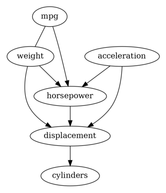
然后我们有一个由PC发现的因果图。让我们也尝试GES来看看它的结果。

from causallearn.search.ScoreBased.GES import ges

# default parameters
Record = ges(data)

# Visualization using pydot
from causallearn.utils.GraphUtils import GraphUtils
import matplotlib.image as mpimg
import matplotlib.pyplot as plt
import io

pyd = GraphUtils.to_pydot(Record['G'], labels=labels)
tmp_png = pyd.create_png(f="png")
fp = io.BytesIO(tmp_png)
img = mpimg.imread(fp, format='png')
plt.axis('off')
plt.imshow(img)
plt.show()

嗯，这两个结果不同，这在将因果发现应用于现实世界数据集时并不罕见，因为对数据生成过程的必要假设很难验证。

此外，PC和GES返回的图是CPDAG而不是DAG，因此可能会有无向边（例如，GES返回的结果）。因此，这些方法的因果效应估计很困难，因为可能缺少后门、工具或前门变量。为了获得DAG，我们决定在我们的数据集上尝试LiNGAM。

from causallearn.search.FCMBased import lingam
model_lingam = lingam.ICALiNGAM()
model_lingam.fit(data)

from causallearn.search.FCMBased.lingam.utils import make_dot
make_dot(model_lingam.adjacency_matrix_, labels=labels)

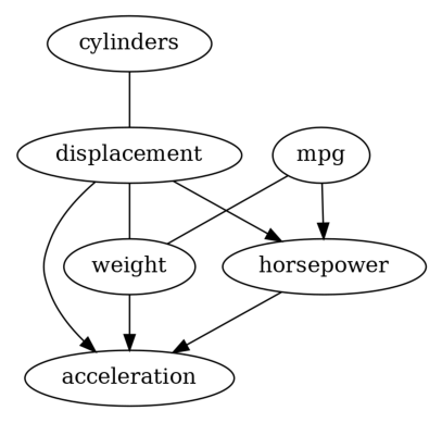
现在我们有了一个DAG，并准备基于它来估计因果效应。

使用线性回归估计因果效应

现在让我们看看mpg对weight的因果效应估计。

# Obtain valid dot format
graph_dot = make_graph(model_lingam.adjacency_matrix_, labels=labels)

# Define Causal Model
model=CausalModel(
        data = data_mpg,
        treatment='mpg',
        outcome='weight',
        graph=str_to_dot(graph_dot.source))

# Identification
identified_estimand = model.identify_effect(proceed_when_unidentifiable=True)
print(identified_estimand)

# Estimation
estimate = model.estimate_effect(identified_estimand,
                                method_name="backdoor.linear_regression",
                                control_value=0,
                                treatment_value=1,
                                confidence_intervals=True,
                                test_significance=True)
print("Causal Estimate is " + str(estimate.value))

Estimand type: EstimandType.NONPARAMETRIC_ATE

### Estimand : 1
Estimand name: backdoor
Estimand expression:
  d
──────(E[weight|cylinders])
d[mpg]
Estimand assumption 1, Unconfoundedness: If U→{mpg} and U→weight then P(weight|mpg,cylinders,U) = P(weight|mpg,cylinders)

### Estimand : 2
Estimand name: iv
No such variable(s) found!

### Estimand : 3
Estimand name: frontdoor
No such variable(s) found!

Causal Estimate is -38.94097365620928

在Sachs数据集上的实验

该数据集包含了对数千个个体免疫系统细胞中11种磷酸化蛋白质和磷脂的同时测量，这些细胞经历了通用和特定的分子干预（Sachs等，2005年）。

数据集的规格如下 - - 节点数量: 11 - 弧线数量: 17 - 参数数量: 178 - 平均马尔可夫毯大小: 3.09 - 平均度数: 3.09 - 最大入度: 3 - 实例数量: 7466

1. 加载数据

from causallearn.utils.Dataset import load_dataset

data_sachs, labels = load_dataset("sachs")

print(data_sachs.shape)
print(labels)

(7466, 11)
['raf', 'mek', 'plc', 'pip2', 'pip3', 'erk', 'akt', 'pka', 'pkc', 'p38', 'jnk']

使用causal-learn进行因果发现

我们使用上述三种因果发现方法（PC、GES和LiNGAM）来寻找因果图。

首先，让我们看一下PC是如何工作的。

graphs = {}
graphs_nx = {}
labels = [f'{col}' for i, col in enumerate(labels)]
data = data_sachs

from causallearn.search.ConstraintBased.PC import pc

cg = pc(data)

# Visualization using pydot
from causallearn.utils.GraphUtils import GraphUtils
import matplotlib.image as mpimg
import matplotlib.pyplot as plt
import io

pyd = GraphUtils.to_pydot(cg.G, labels=labels)
tmp_png = pyd.create_png(f="png")
fp = io.BytesIO(tmp_png)
img = mpimg.imread(fp, format='png')
plt.axis('off')
plt.imshow(img)
plt.show()

然后，让我们尝试GES。

from causallearn.search.ScoreBased.GES import ges

# default parameters
Record = ges(data)

# Visualization using pydot
from causallearn.utils.GraphUtils import GraphUtils
import matplotlib.image as mpimg
import matplotlib.pyplot as plt
import io

pyd = GraphUtils.to_pydot(Record['G'], labels=labels)
tmp_png = pyd.create_png(f="png")
fp = io.BytesIO(tmp_png)
img = mpimg.imread(fp, format='png')
plt.axis('off')
plt.imshow(img)
plt.show()

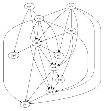
还有LiNGAM。

from causallearn.search.FCMBased import lingam
model = lingam.ICALiNGAM()
model.fit(data)

from causallearn.search.FCMBased.lingam.utils import make_dot
make_dot(model.adjacency_matrix_, labels=labels)

使用线性回归估计效果

同样地，让我们使用LiNGAM返回的DAG来估计PIP2对PKC的因果效应。

# Obtain valid dot format
graph_dot = make_graph(model.adjacency_matrix_, labels=labels)

data_df = pd.DataFrame(data=data, columns=labels)

# Define Causal Model
model_est=CausalModel(
        data = data_df,
        treatment='pip2',
        outcome='pkc',
        graph=str_to_dot(graph_dot.source))

# Identification
identified_estimand = model_est.identify_effect(proceed_when_unidentifiable=False)
print(identified_estimand)

# Estimation
estimate = model_est.estimate_effect(identified_estimand,
                                method_name="backdoor.linear_regression",
                                control_value=0,
                                treatment_value=1,
                                confidence_intervals=True,
                                test_significance=True)
print("Causal Estimate is " + str(estimate.value))

Estimand type: EstimandType.NONPARAMETRIC_ATE

### Estimand : 1
Estimand name: backdoor
Estimand expression:
   d
───────(E[pkc|plc,pip3])
d[pip₂]
Estimand assumption 1, Unconfoundedness: If U→{pip2} and U→pkc then P(pkc|pip2,plc,pip3,U) = P(pkc|pip2,plc,pip3)

### Estimand : 2
Estimand name: iv
No such variable(s) found!

### Estimand : 3
Estimand name: frontdoor
No such variable(s) found!

Causal Estimate is 0.033971892284519356