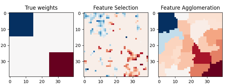
特征聚合与单变量选择

此示例比较了两种降维策略：

• 使用Anova的单变量特征选择

• 使用Ward层次聚类的特征聚合

在回归问题中，使用BayesianRidge作为监督估计器来比较这两种方法。

# 作者：scikit-learn 开发者
# SPDX-License-Identifier: BSD-3-Clause

import shutil
import tempfile

import matplotlib.pyplot as plt
import numpy as np
from joblib import Memory
from scipy import linalg, ndimage

from sklearn import feature_selection
from sklearn.cluster import FeatureAgglomeration
from sklearn.feature_extraction.image import grid_to_graph
from sklearn.linear_model import BayesianRidge
from sklearn.model_selection import GridSearchCV, KFold
from sklearn.pipeline import Pipeline

%% 设置参数

n_samples = 200
size = 40  # image size
roi_size = 15
snr = 5.0
np.random.seed(0)

生成数据

coef = np.zeros((size, size))
coef[0:roi_size, 0:roi_size] = -1.0
coef[-roi_size:, -roi_size:] = 1.0

X = np.random.randn(n_samples, size**2)
for x in X:  # smooth data
    x[:] = ndimage.gaussian_filter(x.reshape(size, size), sigma=1.0).ravel()
X -= X.mean(axis=0)
X /= X.std(axis=0)

y = np.dot(X, coef.ravel())

add noise

noise = np.random.randn(y.shape[0])
noise_coef = (linalg.norm(y, 2) / np.exp(snr / 20.0)) / linalg.norm(noise, 2)
y += noise_coef * noise

计算贝叶斯岭回归的系数并使用网格搜索进行优化

cv = KFold(2)  # cross-validation generator for model selection
ridge = BayesianRidge()
cachedir = tempfile.mkdtemp()
mem = Memory(location=cachedir, verbose=1)

Ward 聚类后接 BayesianRidge

connectivity = grid_to_graph(n_x=size, n_y=size)
ward = FeatureAgglomeration(n_clusters=10, connectivity=connectivity, memory=mem)
clf = Pipeline([("ward", ward), ("ridge", ridge)])
# 通过网格搜索选择最佳包裹数量
clf = GridSearchCV(clf, {"ward__n_clusters": [10, 20, 30]}, n_jobs=1, cv=cv)
clf.fit(X, y)  # set the best parameters
coef_ = clf.best_estimator_.steps[-1][1].coef_
coef_ = clf.best_estimator_.steps[0][1].inverse_transform(coef_)
coef_agglomeration_ = coef_.reshape(size, size)

________________________________________________________________________________
[Memory] Calling sklearn.cluster._agglomerative.ward_tree...
ward_tree(array([[-0.451933, ..., -0.675318],
       ...,
       [ 0.275706, ..., -1.085711]]), connectivity=<COOrdinate sparse matrix of dtype 'int64'
        with 7840 stored elements and shape (1600, 1600)>, n_clusters=None, return_distance=False)
________________________________________________________ward_tree - 0.0s, 0.0min
________________________________________________________________________________
[Memory] Calling sklearn.cluster._agglomerative.ward_tree...
ward_tree(array([[ 0.905206, ...,  0.161245],
       ...,
       [-0.849835, ..., -1.091621]]), connectivity=<COOrdinate sparse matrix of dtype 'int64'
        with 7840 stored elements and shape (1600, 1600)>, n_clusters=None, return_distance=False)
________________________________________________________ward_tree - 0.0s, 0.0min
________________________________________________________________________________
[Memory] Calling sklearn.cluster._agglomerative.ward_tree...
ward_tree(array([[ 0.905206, ..., -0.675318],
       ...,
       [-0.849835, ..., -1.085711]]), connectivity=<COOrdinate sparse matrix of dtype 'int64'
        with 7840 stored elements and shape (1600, 1600)>, n_clusters=None, return_distance=False)
________________________________________________________ward_tree - 0.0s, 0.0min

Anova 单变量特征选择后进行贝叶斯岭回归

f_regression = mem.cache(feature_selection.f_regression)  # caching function
anova = feature_selection.SelectPercentile(f_regression)
clf = Pipeline([("anova", anova), ("ridge", ridge)])
# 选择使用网格搜索的最佳特征百分比
clf = GridSearchCV(clf, {"anova__percentile": [5, 10, 20]}, cv=cv)
clf.fit(X, y)  # set the best parameters
coef_ = clf.best_estimator_.steps[-1][1].coef_
coef_ = clf.best_estimator_.steps[0][1].inverse_transform(coef_.reshape(1, -1))
coef_selection_ = coef_.reshape(size, size)

________________________________________________________________________________
[Memory] Calling sklearn.feature_selection._univariate_selection.f_regression...
f_regression(array([[-0.451933, ...,  0.275706],
       ...,
       [-0.675318, ..., -1.085711]]),
array([ 25.267703, ..., -25.026711]))
_____________________________________________________f_regression - 0.0s, 0.0min
________________________________________________________________________________
[Memory] Calling sklearn.feature_selection._univariate_selection.f_regression...
f_regression(array([[ 0.905206, ..., -0.849835],
       ...,
       [ 0.161245, ..., -1.091621]]),
array([ -27.447268, ..., -112.638768]))
_____________________________________________________f_regression - 0.0s, 0.0min
________________________________________________________________________________
[Memory] Calling sklearn.feature_selection._univariate_selection.f_regression...
f_regression(array([[ 0.905206, ..., -0.849835],
       ...,
       [-0.675318, ..., -1.085711]]),
array([-27.447268, ..., -25.026711]))
_____________________________________________________f_regression - 0.0s, 0.0min

将变换逆转以在图像上绘制结果

plt.close("all")
plt.figure(figsize=(7.3, 2.7))
plt.subplot(1, 3, 1)
plt.imshow(coef, interpolation="nearest", cmap=plt.cm.RdBu_r)
plt.title("True weights")
plt.subplot(1, 3, 2)
plt.imshow(coef_selection_, interpolation="nearest", cmap=plt.cm.RdBu_r)
plt.title("Feature Selection")
plt.subplot(1, 3, 3)
plt.imshow(coef_agglomeration_, interpolation="nearest", cmap=plt.cm.RdBu_r)
plt.title("Feature Agglomeration")
plt.subplots_adjust(0.04, 0.0, 0.98, 0.94, 0.16, 0.26)
plt.show()

尝试删除临时缓存目录，但即使失败也不用担心

shutil.rmtree(cachedir, ignore_errors=True)

Related examples

带有强异常值的数据集上的Huber回归与岭回归对比

带有强异常值的数据集上的Huber回归与岭回归对比

硬币图像的结构化Ward层次聚类演示

硬币图像的结构化Ward层次聚类演示

正交匹配追踪

正交匹配追踪

训练误差与测试误差

训练误差与测试误差