Note

Go to the end to download the full example code. or to run this example in your browser via Binder

使用不同变体的迭代插补法填补缺失值#

IterativeImputer 类非常灵活——它可以与各种估计器一起使用，进行循环回归，依次将每个变量视为输出。

在此示例中，我们比较了一些用于缺失特征插补的估计器与 IterativeImputer ：

BayesianRidge ：正则化线性回归
RandomForestRegressor ：随机树回归森林
make_pipeline (Nystroem , Ridge )：包含二次多项式核扩展和正则化线性回归的管道
KNeighborsRegressor ：与其他 KNN 插补方法相当

特别值得注意的是 IterativeImputer 模拟 missForest 行为的能力，missForest 是 R 语言中一个流行的插补包。

请注意，KNeighborsRegressor 与 KNN 插补不同，后者通过使用考虑缺失值的距离度量从缺失值样本中学习，而不是插补它们。

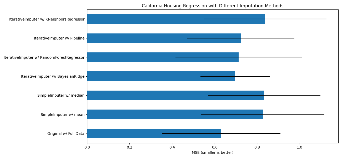
目标是比较不同的估计器，看看在使用 BayesianRidge 估计器对加州房价数据集进行插补时，哪个估计器效果最好，每行随机移除一个值。

对于这种特定的缺失值模式，我们发现 BayesianRidge 和 RandomForestRegressor 给出了最好的结果。

需要注意的是，一些估计器如 HistGradientBoostingRegressor 可以本地处理缺失特征，通常推荐使用这些估计器，而不是构建具有复杂且昂贵的缺失值插补策略的管道。

California Housing Regression with Different Imputation Methods

import matplotlib.pyplot as plt
import numpy as np
import pandas as pd

from sklearn.datasets import fetch_california_housing
from sklearn.ensemble import RandomForestRegressor

# 要使用此实验功能，我们需要明确请求它：
from sklearn.experimental import enable_iterative_imputer  # noqa
from sklearn.impute import IterativeImputer, SimpleImputer
from sklearn.kernel_approximation import Nystroem
from sklearn.linear_model import BayesianRidge, Ridge
from sklearn.model_selection import cross_val_score
from sklearn.neighbors import KNeighborsRegressor
from sklearn.pipeline import make_pipeline

N_SPLITS = 5

rng = np.random.RandomState(0)

X_full, y_full = fetch_california_housing(return_X_y=True)
# 大约2000个样本足以满足示例的目的。
# 删除以下两行代码可以使运行速度变慢，并产生不同的误差条。
X_full = X_full[::10]
y_full = y_full[::10]
n_samples, n_features = X_full.shape

# 估计整个数据集的得分，没有缺失值
br_estimator = BayesianRidge()
score_full_data = pd.DataFrame(
    cross_val_score(
        br_estimator, X_full, y_full, scoring="neg_mean_squared_error", cv=N_SPLITS
    ),
    columns=["Full Data"],
)

# 为每行添加一个缺失值
X_missing = X_full.copy()
y_missing = y_full
missing_samples = np.arange(n_samples)
missing_features = rng.choice(n_features, n_samples, replace=True)
X_missing[missing_samples, missing_features] = np.nan

# 估算填补后的得分（均值和中位数策略）
score_simple_imputer = pd.DataFrame()
for strategy in ("mean", "median"):
    estimator = make_pipeline(
        SimpleImputer(missing_values=np.nan, strategy=strategy), br_estimator
    )
    score_simple_imputer[strategy] = cross_val_score(
        estimator, X_missing, y_missing, scoring="neg_mean_squared_error", cv=N_SPLITS
    )

# 估算使用不同估计器对缺失值进行迭代插补后的得分
estimators = [
    BayesianRidge(),
    RandomForestRegressor(
        # 我们调整了RandomForestRegressor的超参数，以在有限的执行时间内获得足够好的预测性能。
        n_estimators=4,
        max_depth=10,
        bootstrap=True,
        max_samples=0.5,
        n_jobs=2,
        random_state=0,
    ),
    make_pipeline(
        Nystroem(kernel="polynomial", degree=2, random_state=0), Ridge(alpha=1e3)
    ),
    KNeighborsRegressor(n_neighbors=15),
]
score_iterative_imputer = pd.DataFrame()
# 迭代插补器对容差敏感，并依赖于内部使用的估计器。我们调整了容差，以在有限的计算资源下运行此示例，同时与保持容差参数的更严格默认值相比，不会对结果产生太大影响。
tolerances = (1e-3, 1e-1, 1e-1, 1e-2)
for impute_estimator, tol in zip(estimators, tolerances):
    estimator = make_pipeline(
        IterativeImputer(
            random_state=0, estimator=impute_estimator, max_iter=25, tol=tol
        ),
        br_estimator,
    )
    score_iterative_imputer[impute_estimator.__class__.__name__] = cross_val_score(
        estimator, X_missing, y_missing, scoring="neg_mean_squared_error", cv=N_SPLITS
    )

scores = pd.concat(
    [score_full_data, score_simple_imputer, score_iterative_imputer],
    keys=["Original", "SimpleImputer", "IterativeImputer"],
    axis=1,
)

# 绘制加州住房结果
fig, ax = plt.subplots(figsize=(13, 6))
means = -scores.mean()
errors = scores.std()
means.plot.barh(xerr=errors, ax=ax)
ax.set_title("California Housing Regression with Different Imputation Methods")
ax.set_xlabel("MSE (smaller is better)")
ax.set_yticks(np.arange(means.shape[0]))
ax.set_yticklabels([" w/ ".join(label) for label in means.index.tolist()])
plt.tight_layout(pad=1)
plt.show()