Note
Go to the end to download the full example code. or to run this example in your browser via Binder
scikit-learn 0.24 版本发布亮点#
我们很高兴地宣布发布 scikit-learn 0.24 版本!此版本包含了许多错误修复和改进,以及一些新的关键功能。以下是本次发布的一些主要功能。 有关所有更改的详尽列表 ,请参阅 发布说明 。
要安装最新版本(使用 pip):
pip install --upgrade scikit-learn
或使用 conda:
conda install -c conda-forge scikit-learn
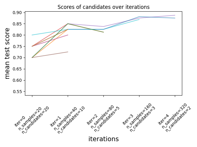
连续减半估计器用于调优超参数#
连续减半法,一种先进的方法,现在可以用来探索参数空间并识别其最佳组合。
HalvingGridSearchCV 和
HalvingRandomSearchCV 可以作为
GridSearchCV 和
RandomizedSearchCV 的直接替代品。
连续减半法是一个迭代选择过程,如下图所示。第一次迭代使用少量资源运行,
这些资源通常对应于训练样本的数量,但也可以是一个任意的整数参数,
例如随机森林中的 n_estimators 。只有一部分参数候选者会被选中进入下一次迭代,
下一次迭代将分配更多的资源。只有一部分候选者会持续到迭代过程的最后,
得分最高的参数候选者就是最后一次迭代中的最佳参数候选者。
请参阅 用户指南 了解更多信息(注意:逐次缩减估计器仍然是 实验性的 )。
- target:
../model_selection/plot_successive_halving_iterations.html
- align:
center
import numpy as np
from scipy.stats import randint
from sklearn.experimental import enable_halving_search_cv  # noqa
from sklearn.model_selection import HalvingRandomSearchCV
from sklearn.ensemble import RandomForestClassifier
from sklearn.datasets import make_classification

rng = np.random.RandomState(0)

X, y = make_classification(n_samples=700, random_state=rng)

clf = RandomForestClassifier(n_estimators=10, random_state=rng)

param_dist = {
    "max_depth": [3, None],
    "max_features": randint(1, 11),
    "min_samples_split": randint(2, 11),
    "bootstrap": [True, False],
    "criterion": ["gini", "entropy"],
}

rsh = HalvingRandomSearchCV(
    estimator=clf, param_distributions=param_dist, factor=2, random_state=rng
)
rsh.fit(X, y)
rsh.best_params_
{'bootstrap': True, 'criterion': 'gini', 'max_depth': None, 'max_features': 10, 'min_samples_split': 10}
对分类特征在直方图梯度提升估计器中的原生支持#
HistGradientBoostingClassifier 和
HistGradientBoostingRegressor 现在对分类特征有了原生支持:它们可以考虑对无序的分类数据进行分裂。请在 用户指南 中阅读更多内容。

- target:
../ensemble/plot_gradient_boosting_categorical.html
- align:
center
该图显示了对分类特征的新原生支持导致拟合时间与将类别视为有序数量(即简单的序数编码)处理的模型相当。原生支持也比独热编码和序数编码更具表现力。然而,要使用新的 categorical_features 参数,仍然需要在管道中预处理数据,如此 示例 所示。
提升了HistGradientBoosting估计器的性能#
在调用 fit 时,ensemble.HistGradientBoostingRegressor 和
ensemble.HistGradientBoostingClassifier 的内存占用显著减少。此外,
直方图初始化现在是并行进行的,从而带来了轻微的速度提升。
更多信息请参见 基准测试页面 。
新的自训练元估计器#
基于 Yarowski’s algorithm 的新自训练实现现在可以与任何实现了 predict_proba 的分类器一起使用。子分类器将表现为一个半监督分类器,使其能够从未标记的数据中学习。更多内容请参阅 用户指南 。
import numpy as np
from sklearn import datasets
from sklearn.semi_supervised import SelfTrainingClassifier
from sklearn.svm import SVC

rng = np.random.RandomState(42)
iris = datasets.load_iris()
random_unlabeled_points = rng.rand(iris.target.shape[0]) < 0.3
iris.target[random_unlabeled_points] = -1
svc = SVC(probability=True, gamma="auto")
self_training_model = SelfTrainingClassifier(svc)
self_training_model.fit(iris.data, iris.target)
新的SequentialFeatureSelector转换器#
一个新的迭代转换器用于选择特征:
SequentialFeatureSelector 。
顺序特征选择可以一次添加一个特征(前向选择)或从可用特征列表中删除特征(后向选择),基于交叉验证得分最大化。
请参阅 用户指南 。
from sklearn.feature_selection import SequentialFeatureSelector
from sklearn.neighbors import KNeighborsClassifier
from sklearn.datasets import load_iris

X, y = load_iris(return_X_y=True, as_frame=True)
feature_names = X.columns
knn = KNeighborsClassifier(n_neighbors=3)
sfs = SequentialFeatureSelector(knn, n_features_to_select=2)
sfs.fit(X, y)
print(
    "Features selected by forward sequential selection: "
    f"{feature_names[sfs.get_support()].tolist()}"
)
Features selected by forward sequential selection: ['sepal length (cm)', 'petal width (cm)']
新的 PolynomialCountSketch 核近似函数#
新的 PolynomialCountSketch 在与线性模型一起使用时,近似于特征空间的多项式扩展,但比 PolynomialFeatures 使用的内存少得多。
from sklearn.datasets import fetch_covtype
from sklearn.pipeline import make_pipeline
from sklearn.model_selection import train_test_split
from sklearn.preprocessing import MinMaxScaler
from sklearn.kernel_approximation import PolynomialCountSketch
from sklearn.linear_model import LogisticRegression

X, y = fetch_covtype(return_X_y=True)
pipe = make_pipeline(
    MinMaxScaler(),
    PolynomialCountSketch(degree=2, n_components=300),
    LogisticRegression(max_iter=1000),
)
X_train, X_test, y_train, y_test = train_test_split(
    X, y, train_size=5000, test_size=10000, random_state=42
)
pipe.fit(X_train, y_train).score(X_test, y_test)
0.7361
为了比较,以下是相同数据的线性基线得分:
linear_baseline = make_pipeline(MinMaxScaler(), LogisticRegression(max_iter=1000))
linear_baseline.fit(X_train, y_train).score(X_test, y_test)
0.7141
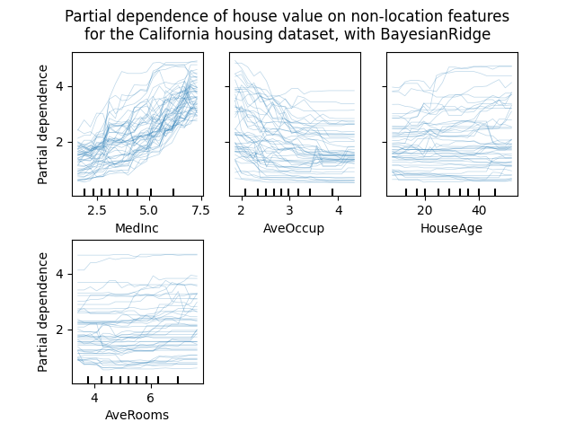
个体条件期望图#
一种新的部分依赖图现已推出:个体条件期望(ICE)图。ICE 图分别可视化每个样本的预测对某个特征的依赖性,每个样本对应一条线。 请参阅:用户指南 <individual_conditional>
from sklearn.ensemble import RandomForestRegressor
from sklearn.datasets import fetch_california_housing

# from sklearn.inspection import plot_partial_dependence
from sklearn.inspection import PartialDependenceDisplay

X, y = fetch_california_housing(return_X_y=True, as_frame=True)
features = ["MedInc", "AveOccup", "HouseAge", "AveRooms"]
est = RandomForestRegressor(n_estimators=10)
est.fit(X, y)

# plot_partial_dependence 已在版本 1.2 中被移除。从 1.2 开始,请使用 PartialDependenceDisplay 代替。
# display = plot_partial_dependence(
display = PartialDependenceDisplay.from_estimator(
    est,
    X,
    features,
    kind="individual",
    subsample=50,
    n_jobs=3,
    grid_resolution=20,
    random_state=0,
)
display.figure_.suptitle(
    "Partial dependence of house value on non-location features\n"
    "for the California housing dataset, with BayesianRidge"
)
display.figure_.subplots_adjust(hspace=0.3)
新的泊松分裂标准用于DecisionTreeRegressor#
泊松回归估计的集成从0.23版本继续。
DecisionTreeRegressor 现在支持新的 'poisson'
分裂标准。如果你的目标是计数或频率,设置 criterion="poisson" 可能是一个不错的选择。
from sklearn.tree import DecisionTreeRegressor
from sklearn.model_selection import train_test_split
import numpy as np

n_samples, n_features = 1000, 20
rng = np.random.RandomState(0)
X = rng.randn(n_samples, n_features)
# 与X[:, 5]相关的正整数目标,包含许多零:
y = rng.poisson(lam=np.exp(X[:, 5]) / 2)
X_train, X_test, y_train, y_test = train_test_split(X, y, random_state=rng)
regressor = DecisionTreeRegressor(criterion="poisson", random_state=0)
regressor.fit(X_train, y_train)
新的文档改进#
新增了示例和文档页面,以持续改进对机器学习实践的理解:
一个关于 常见陷阱和推荐实践 的新章节,
一个示例,说明如何 统计比较模型性能 ,使用
GridSearchCV进行评估,一个示例,说明如何 解释线性模型的系数 ,
一个 示例 比较主成分回归和偏最小二乘法。
Total running time of the script: (0 minutes 11.558 seconds)
Related examples