Note
Go to the end to download the full example code. or to run this example in your browser via Binder
理解决策树结构#
可以分析决策树结构,以进一步了解特征与预测目标之间的关系。在这个例子中,我们展示了如何获取:
二叉树结构;
每个节点的深度以及它是否是叶节点;
使用
decision_path方法由样本到达的节点;使用apply方法由样本到达的叶节点;
用于预测样本的规则;
一组样本共享的决策路径。
import numpy as np
from matplotlib import pyplot as plt

from sklearn import tree
from sklearn.datasets import load_iris
from sklearn.model_selection import train_test_split
from sklearn.tree import DecisionTreeClassifier
训练树分类器#
首先,我们使用 load_iris 数据集拟合一个 DecisionTreeClassifier 。
iris = load_iris()
X = iris.data
y = iris.target
X_train, X_test, y_train, y_test = train_test_split(X, y, random_state=0)

clf = DecisionTreeClassifier(max_leaf_nodes=3, random_state=0)
clf.fit(X_train, y_train)
树结构#
决策分类器有一个名为 tree_ 的属性,可以访问低级属性,如节点总数 node_count 和树的最大深度 max_depth 。 tree_.compute_node_depths() 方法计算树中每个节点的深度。 tree_ 还存储整个二叉树结构,表示为多个并行数组。每个数组的第i个元素包含关于节点 i 的信息。节点0是树的根节点。一些数组仅适用于叶节点或分裂节点。在这种情况下,另一种类型节点的值是任意的。例如,数组 feature 和 threshold 仅适用于分裂节点。因此,这些数组中叶节点的值是任意的。
在这些数组中,我们有:
children_left[i]:节点i的左子节点的 id,若为叶节点则为 -1children_right[i]:节点i的右子节点的 id,若为叶节点则为 -1feature[i]:用于分裂节点i的特征threshold[i]:节点i的阈值n_node_samples[i]:到达节点i的训练样本数量impurity[i]:节点i的不纯度weighted_n_node_samples[i]:到达节点i的加权训练样本数量value[i, j, k]:到达节点 i 的训练样本在输出 j 和类别 k 上的汇总(对于回归树,类别设为 1)。有关value的更多信息,请参见下文。
使用数组,我们可以遍历树结构来计算各种属性。下面,我们将计算每个节点的深度以及它是否是叶子节点。
n_nodes = clf.tree_.node_count
children_left = clf.tree_.children_left
children_right = clf.tree_.children_right
feature = clf.tree_.feature
threshold = clf.tree_.threshold
values = clf.tree_.value

node_depth = np.zeros(shape=n_nodes, dtype=np.int64)
is_leaves = np.zeros(shape=n_nodes, dtype=bool)
stack = [(0, 0)]  # start with the root node id (0) and its depth (0)
while len(stack) > 0:
    # `pop` 确保每个节点只被访问一次
    node_id, depth = stack.pop()
    node_depth[node_id] = depth

    # 如果一个节点的左子节点和右子节点不同,我们就有一个分裂节点
    is_split_node = children_left[node_id] != children_right[node_id]
    # 如果是一个分裂节点,将左子节点和右子节点及其深度添加到 `stack` 中,以便我们可以遍历它们
    if is_split_node:
        stack.append((children_left[node_id], depth + 1))
        stack.append((children_right[node_id], depth + 1))
    else:
        is_leaves[node_id] = True

print(
    "The binary tree structure has {n} nodes and has "
    "the following tree structure:\n".format(n=n_nodes)
)
for i in range(n_nodes):
    if is_leaves[i]:
        print(
            "{space}node={node} is a leaf node with value={value}.".format(
                space=node_depth[i] * "\t", node=i, value=np.around(values[i], 3)
            )
        )
    else:
        print(
            "{space}node={node} is a split node with value={value}: "
            "go to node {left} if X[:, {feature}] <= {threshold} "
            "else to node {right}.".format(
                space=node_depth[i] * "\t",
                node=i,
                left=children_left[i],
                feature=feature[i],
                threshold=threshold[i],
                right=children_right[i],
                value=np.around(values[i], 3),
            )
        )
The binary tree structure has 5 nodes and has the following tree structure:

node=0 is a split node with value=[[0.33  0.304 0.366]]: go to node 1 if X[:, 3] <= 0.800000011920929 else to node 2.
        node=1 is a leaf node with value=[[1. 0. 0.]].
        node=2 is a split node with value=[[0.    0.453 0.547]]: go to node 3 if X[:, 2] <= 4.950000047683716 else to node 4.
                node=3 is a leaf node with value=[[0.    0.917 0.083]].
                node=4 is a leaf node with value=[[0.    0.026 0.974]].
这里使用的 values 数组是什么?#
tree_.value 数组是一个形状为 [ n_nodes , n_classes , n_outputs ] 的三维数组,
它提供了到达每个节点的样本在每个类别和每个输出上的比例。
每个节点都有一个 value 数组,该数组表示相对于父节点到达该节点的加权样本在每个输出和类别上的比例。
可以通过将该数字乘以给定节点的 tree_.weighted_n_node_samples[node_idx] 来将其转换为到达节点的绝对加权样本数。注意,在此示例中未使用样本权重,因此加权样本数即为到达节点的样本数,因为每个样本默认权重为1。
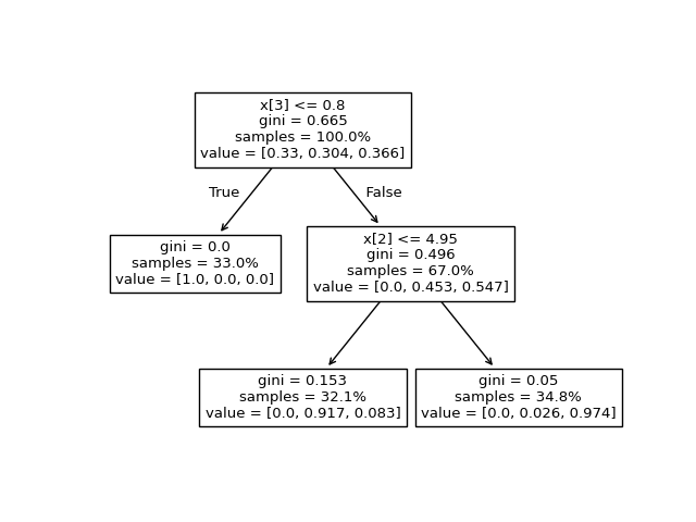
例如,在上面基于鸢尾花数据集构建的树中,根节点的 value = [0.33, 0.304, 0.366] 表示在根节点有33%的类别0样本,30.4%的类别1样本和36.6%的类别2样本。可以通过乘以到达根节点的样本数量 tree_.weighted_n_node_samples[0] 将其转换为绝对样本数量。然后根节点的 value = [37, 34, 41] 表示在根节点有37个类别0样本,34个类别1样本和41个类别2样本。
遍历树时,样本会被分割,因此到达每个节点的 value 数组会发生变化。根节点的左子节点的 value = [1., 0, 0] (或转换为绝对样本数时为 value = [37, 0, 0] ),因为左子节点中的所有37个样本都来自类别0。
注意:在这个例子中, n_outputs=1 ,但树分类器也可以处理多输出问题。每个节点的 value 数组将只是一个二维数组。
我们可以将上述输出与决策树的图进行比较。在这里,我们展示了到达每个节点的每个类别样本的比例,这些节点对应于 tree_.value 数组的实际元素。
tree.plot_tree(clf, proportion=True)
plt.show()
决策路径#
我们还可以检索感兴趣样本的决策路径。 decision_path 方法输出一个指示矩阵,使我们能够检索样本经过的节点。指示矩阵中位置 (i, j) 的非零元素表示样本 i 经过节点 j 。或者,对于一个样本 i ,指示矩阵第 i 行中非零元素的位置表示该样本经过的节点的 ID。
可以使用 apply 方法获取感兴趣样本到达的叶子节点ID。该方法返回一个数组,其中包含每个感兴趣样本到达的叶子节点的ID。利用叶子节点ID和 decision_path ,我们可以获得用于预测单个样本或一组样本的分裂条件。首先,让我们对一个样本进行操作。请注意, node_index 是一个稀疏矩阵。
node_indicator = clf.decision_path(X_test)
leaf_id = clf.apply(X_test)

sample_id = 0
# 获取 `sample_id` 经过的节点 ID,即第 `sample_id` 行
node_index = node_indicator.indices[
    node_indicator.indptr[sample_id] : node_indicator.indptr[sample_id + 1]
]

print("Rules used to predict sample {id}:\n".format(id=sample_id))
for node_id in node_index:
    # 如果是叶节点,则继续到下一个节点
    if leaf_id[sample_id] == node_id:
        continue

    # 检查样本0的分裂特征值是否低于阈值
    if X_test[sample_id, feature[node_id]] <= threshold[node_id]:
        threshold_sign = "<="
    else:
        threshold_sign = ">"

    print(
        "decision node {node} : (X_test[{sample}, {feature}] = {value}) "
        "{inequality} {threshold})".format(
            node=node_id,
            sample=sample_id,
            feature=feature[node_id],
            value=X_test[sample_id, feature[node_id]],
            inequality=threshold_sign,
            threshold=threshold[node_id],
        )
    )
Rules used to predict sample 0:

decision node 0 : (X_test[0, 3] = 2.4) > 0.800000011920929)
decision node 2 : (X_test[0, 2] = 5.1) > 4.950000047683716)
对于一组样本,我们可以确定这些样本经过的共同节点。
sample_ids = [0, 1]
# 表示两个样本都经过的节点的布尔数组
common_nodes = node_indicator.toarray()[sample_ids].sum(axis=0) == len(sample_ids)
# 使用数组中的位置获取节点ID
common_node_id = np.arange(n_nodes)[common_nodes]

print(
    "\nThe following samples {samples} share the node(s) {nodes} in the tree.".format(
        samples=sample_ids, nodes=common_node_id
    )
)
print("This is {prop}% of all nodes.".format(prop=100 * len(common_node_id) / n_nodes))
The following samples [0, 1] share the node(s) [0 2] in the tree.
This is 40.0% of all nodes.
Total running time of the script: (0 minutes 0.041 seconds)
Related examples