Note
Go to the end to download the full example code. or to run this example in your browser via Binder
介绍 set_output API#
- 本示例将演示
set_outputAPI 以配置转换器输出 pandas DataFrame。set_output可以通过调用set_output方法为每个估计器单独配置,也可以通过设置set_config(transform_output="pandas")全局配置。详情请参见 SLEP018 _。
首先,我们将鸢尾花数据集加载为一个 DataFrame,以演示 set_output API。
from sklearn.datasets import load_iris
from sklearn.model_selection import train_test_split

X, y = load_iris(as_frame=True, return_X_y=True)
X_train, X_test, y_train, y_test = train_test_split(X, y, stratify=y, random_state=0)
X_train.head()
要配置估计器(例如 preprocessing.StandardScaler )以返回 DataFrame,请调用 set_output 。此功能需要安装 pandas。
from sklearn.preprocessing import StandardScaler

scaler = StandardScaler().set_output(transform="pandas")

scaler.fit(X_train)
X_test_scaled = scaler.transform(X_test)
X_test_scaled.head()
set_output 可以在 fit 之后调用,以便在事后配置 transform 。
scaler2 = StandardScaler()

scaler2.fit(X_train)
X_test_np = scaler2.transform(X_test)
print(f"Default output type: {type(X_test_np).__name__}")

scaler2.set_output(transform="pandas")
X_test_df = scaler2.transform(X_test)
print(f"Configured pandas output type: {type(X_test_df).__name__}")
Default output type: ndarray
Configured pandas output type: DataFrame
在 pipeline.Pipeline 中, set_output 将所有步骤配置为输出 DataFrame。
from sklearn.feature_selection import SelectPercentile
from sklearn.linear_model import LogisticRegression
from sklearn.pipeline import make_pipeline

clf = make_pipeline(
    StandardScaler(), SelectPercentile(percentile=75), LogisticRegression()
)
clf.set_output(transform="pandas")
clf.fit(X_train, y_train)
每个管道中的转换器都被配置为返回数据框。这意味着最终的逻辑回归步骤包含输入的特征名称。
clf[-1].feature_names_in_
array(['sepal length (cm)', 'petal length (cm)', 'petal width (cm)'],
      dtype=object)
Note
如果使用 set_params 方法,转换器将被替换为具有默认输出格式的新转换器。
clf.set_params(standardscaler=StandardScaler())
clf.fit(X_train, y_train)
clf[-1].feature_names_in_
array(['x0', 'x2', 'x3'], dtype=object)
为了保持预期行为,请事先在新的转换器上使用 set_output 。
scaler = StandardScaler().set_output(transform="pandas")
clf.set_params(standardscaler=scaler)
clf.fit(X_train, y_train)
clf[-1].feature_names_in_
array(['sepal length (cm)', 'petal length (cm)', 'petal width (cm)'],
      dtype=object)
接下来我们加载泰坦尼克号数据集,以演示 set_output 与 compose.ColumnTransformer 和异构数据的结合使用。
from sklearn.datasets import fetch_openml

X, y = fetch_openml("titanic", version=1, as_frame=True, return_X_y=True)
X_train, X_test, y_train, y_test = train_test_split(X, y, stratify=y)
可以通过使用 set_config 并将 transform_output 设置为 "pandas" 来全局配置 set_output API。
from sklearn import set_config
from sklearn.compose import ColumnTransformer
from sklearn.impute import SimpleImputer
from sklearn.preprocessing import OneHotEncoder, StandardScaler

set_config(transform_output="pandas")

num_pipe = make_pipeline(SimpleImputer(), StandardScaler())
num_cols = ["age", "fare"]
ct = ColumnTransformer(
    (
        ("numerical", num_pipe, num_cols),
        (
            "categorical",
            OneHotEncoder(
                sparse_output=False, drop="if_binary", handle_unknown="ignore"
            ),
            ["embarked", "sex", "pclass"],
        ),
    ),
    verbose_feature_names_out=False,
)
clf = make_pipeline(ct, SelectPercentile(percentile=50), LogisticRegression())
clf.fit(X_train, y_train)
clf.score(X_test, y_test)
0.7865853658536586
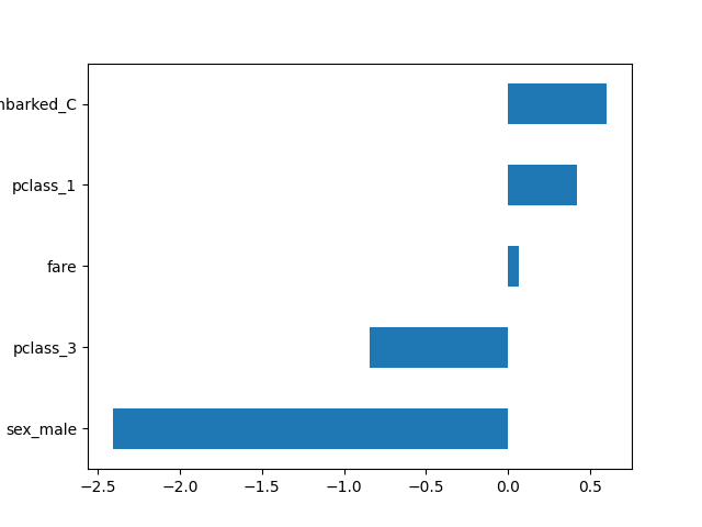
通过全局配置,所有转换器输出DataFrame。这使我们能够轻松地绘制逻辑回归系数及其对应的特征名称。
import pandas as pd

log_reg = clf[-1]
coef = pd.Series(log_reg.coef_.ravel(), index=log_reg.feature_names_in_)
_ = coef.sort_values().plot.barh()
为了演示下面的 config_context 功能,让我们首先将 transform_output 重置为默认值。
set_config(transform_output="default")
在使用 config_context 配置输出类型时,以调用 transform 或 fit_transform 时的配置为准。仅在构造或拟合转换器时设置这些配置是无效的。
from sklearn import config_context

scaler = StandardScaler()
scaler.fit(X_train[num_cols])
with config_context(transform_output="pandas"):
    # transform 的输出将是一个 Pandas DataFrame
    X_test_scaled = scaler.transform(X_test[num_cols])
X_test_scaled.head()
在上下文管理器之外,输出将是一个 NumPy 数组
X_test_scaled = scaler.transform(X_test[num_cols])
X_test_scaled[:5]
array([[-0.74528776, -0.34389503],
       [        nan,  0.85164139],
       [-0.05589876, -0.48727316],
       [-0.81422666,  0.45262953],
       [-0.60740996, -0.48644889]])
Total running time of the script: (0 minutes 0.088 seconds)
Related examples