Note

Go to the end to download the full example code. or to run this example in your browser via Binder

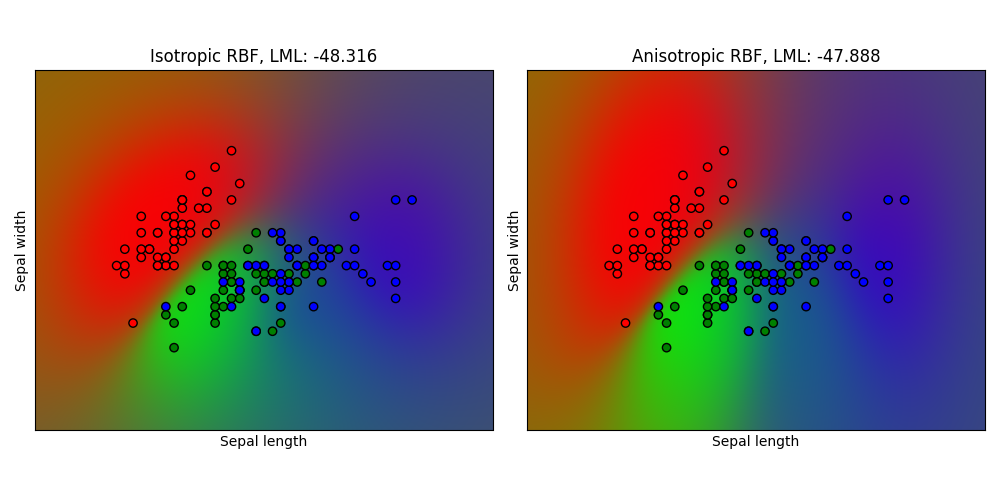
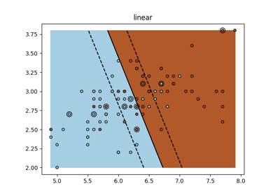
基于高斯过程分类（GPC）的鸢尾花数据集#

本示例展示了在鸢尾花数据集的二维版本上，使用各向同性和各向异性RBF核的GPC预测概率。各向异性RBF核通过为两个特征维度分配不同的长度尺度，获得了略高的对数边际似然。

Isotropic RBF, LML: -48.316, Anisotropic RBF, LML: -47.888

import matplotlib.pyplot as plt
import numpy as np

from sklearn import datasets
from sklearn.gaussian_process import GaussianProcessClassifier
from sklearn.gaussian_process.kernels import RBF

# 导入一些数据来玩玩
iris = datasets.load_iris()
X = iris.data[:, :2]  # we only take the first two features.
y = np.array(iris.target, dtype=int)

h = 0.02  # step size in the mesh

kernel = 1.0 * RBF([1.0])
gpc_rbf_isotropic = GaussianProcessClassifier(kernel=kernel).fit(X, y)
kernel = 1.0 * RBF([1.0, 1.0])
gpc_rbf_anisotropic = GaussianProcessClassifier(kernel=kernel).fit(X, y)

# 创建一个网格进行绘图
x_min, x_max = X[:, 0].min() - 1, X[:, 0].max() + 1
y_min, y_max = X[:, 1].min() - 1, X[:, 1].max() + 1
xx, yy = np.meshgrid(np.arange(x_min, x_max, h), np.arange(y_min, y_max, h))

titles = ["Isotropic RBF", "Anisotropic RBF"]
plt.figure(figsize=(10, 5))
for i, clf in enumerate((gpc_rbf_isotropic, gpc_rbf_anisotropic)):
    # 绘制预测概率。为此，我们将为网格 [x_min, x_max]x[y_min, y_max] 中的每个点分配一个颜色。
    plt.subplot(1, 2, i + 1)

    Z = clf.predict_proba(np.c_[xx.ravel(), yy.ravel()])

    # 将结果放入彩色图中
    Z = Z.reshape((xx.shape[0], xx.shape[1], 3))
    plt.imshow(Z, extent=(x_min, x_max, y_min, y_max), origin="lower")

    # 还要绘制训练点
    plt.scatter(X[:, 0], X[:, 1], c=np.array(["r", "g", "b"])[y], edgecolors=(0, 0, 0))
    plt.xlabel("Sepal length")
    plt.ylabel("Sepal width")
    plt.xlim(xx.min(), xx.max())
    plt.ylim(yy.min(), yy.max())
    plt.xticks(())
    plt.yticks(())
    plt.title(
        "%s, LML: %.3f" % (titles[i], clf.log_marginal_likelihood(clf.kernel_.theta))
    )

plt.tight_layout()
plt.show()