Note

Go to the end to download the full example code. or to run this example in your browser via Binder

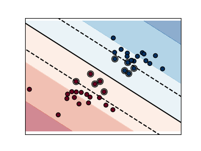
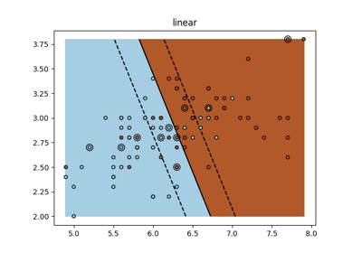
SVM 边界示例#

下图说明了参数 C 对分隔线的影响。 C 的值较大时，基本上告诉我们的模型我们对数据的分布没有太多信心，只会考虑靠近分隔线的点。

C 的值较小时，会包含更多/所有的观测值，允许使用该区域内的所有数据来计算边界。

# 代码来源：Gaël Varoquaux
# 由Jaques Grobler修改用于文档
# SPDX许可证标识符：BSD-3-Clause

import matplotlib.pyplot as plt
import numpy as np

from sklearn import svm

# 我们创建了40个可分离点
np.random.seed(0)
X = np.r_[np.random.randn(20, 2) - [2, 2], np.random.randn(20, 2) + [2, 2]]
Y = [0] * 20 + [1] * 20

# 图号
fignum = 1

# 拟合模型
for name, penalty in (("unreg", 1), ("reg", 0.05)):
    clf = svm.SVC(kernel="linear", C=penalty)
    clf.fit(X, Y)

    # 获取分离超平面
    w = clf.coef_[0]
    a = -w[0] / w[1]
    xx = np.linspace(-5, 5)
    yy = a * xx - (clf.intercept_[0]) / w[1]

    # 绘制通过支持向量的平行于分离超平面的直线（在垂直于超平面的方向上距离超平面一个边距）。在二维中，这个距离是垂直方向上的 sqrt(1+a^2)。
    margin = 1 / np.sqrt(np.sum(clf.coef_**2))
    yy_down = yy - np.sqrt(1 + a**2) * margin
    yy_up = yy + np.sqrt(1 + a**2) * margin

    # 绘制直线、点和最近的向量到平面
    plt.figure(fignum, figsize=(4, 3))
    plt.clf()
    plt.plot(xx, yy, "k-")
    plt.plot(xx, yy_down, "k--")
    plt.plot(xx, yy_up, "k--")

    plt.scatter(
        clf.support_vectors_[:, 0],
        clf.support_vectors_[:, 1],
        s=80,
        facecolors="none",
        zorder=10,
        edgecolors="k",
    )
    plt.scatter(
        X[:, 0], X[:, 1], c=Y, zorder=10, cmap=plt.get_cmap("RdBu"), edgecolors="k"
    )

    plt.axis("tight")
    x_min = -4.8
    x_max = 4.2
    y_min = -6
    y_max = 6

    YY, XX = np.meshgrid(yy, xx)
    xy = np.vstack([XX.ravel(), YY.ravel()]).T
    Z = clf.decision_function(xy).reshape(XX.shape)

    # 将结果放入轮廓图中
    plt.contourf(XX, YY, Z, cmap=plt.get_cmap("RdBu"), alpha=0.5, linestyles=["-"])

    plt.xlim(x_min, x_max)
    plt.ylim(y_min, y_max)

    plt.xticks(())
    plt.yticks(())
    fignum = fignum + 1

plt.show()