Note

Go to the end to download the full example code. or to run this example in your browser via Binder

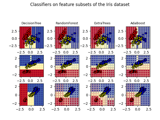
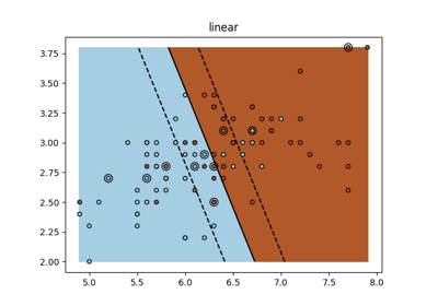
绘制鸢尾花数据集上树集成的决策边界#

绘制在鸢尾花数据集的特征对上训练的随机树森林的决策边界。

此图比较了决策树分类器（第一列）、随机森林分类器（第二列）、极端随机树分类器（第三列）和AdaBoost分类器（第四列）学习到的决策边界。

在第一行中，分类器仅使用花萼宽度和花萼长度特征构建；在第二行中，仅使用花瓣长度和花萼长度特征构建；在第三行中，仅使用花瓣宽度和花瓣长度特征构建。

按质量降序排列，当在所有4个特征上使用30个估计器进行训练并使用10折交叉验证评分时，我们看到：

ExtraTreesClassifier() # 0.95分 RandomForestClassifier() # 0.94分 AdaBoost(DecisionTree(max_depth=3)) # 0.94分 DecisionTree(max_depth=None) # 0.94分

增加AdaBoost的 max_depth 会降低分数的标准差（但平均分数不会提高）。

有关每个模型的更多详细信息，请参见控制台输出。

在此示例中，您可以尝试：

改变 DecisionTreeClassifier 和 AdaBoostClassifier 的 max_depth ，例如尝试 DecisionTreeClassifier 的 max_depth=3 或 AdaBoostClassifier 的 max_depth=None
改变 n_estimators

值得注意的是，随机森林和极端随机树可以在多核上并行拟合，因为每棵树是独立构建的。AdaBoost的样本是顺序构建的，因此不使用多核。

Classifiers on feature subsets of the Iris dataset, DecisionTree, RandomForest, ExtraTrees, AdaBoost

DecisionTree with features [0, 1] has a score of 0.9266666666666666
RandomForest with 30 estimators with features [0, 1] has a score of 0.9266666666666666
ExtraTrees with 30 estimators with features [0, 1] has a score of 0.9266666666666666
AdaBoost with 30 estimators with features [0, 1] has a score of 0.82
DecisionTree with features [0, 2] has a score of 0.9933333333333333
RandomForest with 30 estimators with features [0, 2] has a score of 0.9933333333333333
ExtraTrees with 30 estimators with features [0, 2] has a score of 0.9933333333333333
AdaBoost with 30 estimators with features [0, 2] has a score of 0.9933333333333333
DecisionTree with features [2, 3] has a score of 0.9933333333333333
RandomForest with 30 estimators with features [2, 3] has a score of 0.9933333333333333
ExtraTrees with 30 estimators with features [2, 3] has a score of 0.9933333333333333
AdaBoost with 30 estimators with features [2, 3] has a score of 0.9866666666666667

import matplotlib.pyplot as plt
import numpy as np
from matplotlib.colors import ListedColormap

from sklearn.datasets import load_iris
from sklearn.ensemble import (
    AdaBoostClassifier,
    ExtraTreesClassifier,
    RandomForestClassifier,
)
from sklearn.tree import DecisionTreeClassifier

# Parameters
n_classes = 3
n_estimators = 30
cmap = plt.cm.RdYlBu
plot_step = 0.02  # fine step width for decision surface contours
plot_step_coarser = 0.5  # step widths for coarse classifier guesses
RANDOM_SEED = 13  # fix the seed on each iteration

# Load data
iris = load_iris()

plot_idx = 1

models = [
    DecisionTreeClassifier(max_depth=None),
    RandomForestClassifier(n_estimators=n_estimators),
    ExtraTreesClassifier(n_estimators=n_estimators),
    AdaBoostClassifier(
        DecisionTreeClassifier(max_depth=3),
        n_estimators=n_estimators,
        algorithm="SAMME",
    ),
]

for pair in ([0, 1], [0, 2], [2, 3]):
    for model in models:
        # 我们只取两个对应的特征
        X = iris.data[:, pair]
        y = iris.target

        # Shuffle
        idx = np.arange(X.shape[0])
        np.random.seed(RANDOM_SEED)
        np.random.shuffle(idx)
        X = X[idx]
        y = y[idx]

        # 标准化
        mean = X.mean(axis=0)
        std = X.std(axis=0)
        X = (X - mean) / std

        # Train
        model.fit(X, y)

        scores = model.score(X, y)
        # 为每个列和控制台创建一个标题，使用 str() 并切掉字符串中无用的部分
        model_title = str(type(model)).split(".")[-1][:-2][: -len("Classifier")]

        model_details = model_title
        if hasattr(model, "estimators_"):
            model_details += " with {} estimators".format(len(model.estimators_))
        print(model_details + " with features", pair, "has a score of", scores)

        plt.subplot(3, 4, plot_idx)
        if plot_idx <= len(models):
            # 在每列的顶部添加一个标题
            plt.title(model_title, fontsize=9)

        # 现在使用细网格作为输入绘制决策边界，并生成填充轮廓图
        x_min, x_max = X[:, 0].min() - 1, X[:, 0].max() + 1
        y_min, y_max = X[:, 1].min() - 1, X[:, 1].max() + 1
        xx, yy = np.meshgrid(
            np.arange(x_min, x_max, plot_step), np.arange(y_min, y_max, plot_step)
        )

        # 绘制单个DecisionTreeClassifier或对分类器集成的决策边界进行alpha混合
        if isinstance(model, DecisionTreeClassifier):
            Z = model.predict(np.c_[xx.ravel(), yy.ravel()])
            Z = Z.reshape(xx.shape)
            cs = plt.contourf(xx, yy, Z, cmap=cmap)
        else:
            # 选择 alpha 混合级别时要考虑正在使用的估计器数量（需要注意的是，如果 AdaBoost 提前达到了足够好的拟合效果，它可以使用比最大数量更少的估计器）。
            estimator_alpha = 1.0 / len(model.estimators_)
            for tree in model.estimators_:
                Z = tree.predict(np.c_[xx.ravel(), yy.ravel()])
                Z = Z.reshape(xx.shape)
                cs = plt.contourf(xx, yy, Z, alpha=estimator_alpha, cmap=cmap)

        # 构建一个更粗略的网格来绘制一组集成分类，以展示这些分类与我们在决策边界中看到的有何不同。这些点是规则分布的，并且没有黑色轮廓。
        xx_coarser, yy_coarser = np.meshgrid(
            np.arange(x_min, x_max, plot_step_coarser),
            np.arange(y_min, y_max, plot_step_coarser),
        )
        Z_points_coarser = model.predict(
            np.c_[xx_coarser.ravel(), yy_coarser.ravel()]
        ).reshape(xx_coarser.shape)
        cs_points = plt.scatter(
            xx_coarser,
            yy_coarser,
            s=15,
            c=Z_points_coarser,
            cmap=cmap,
            edgecolors="none",
        )

        # 绘制训练点，这些点聚集在一起并有黑色轮廓。
        plt.scatter(
            X[:, 0],
            X[:, 1],
            c=y,
            cmap=ListedColormap(["r", "y", "b"]),
            edgecolor="k",
            s=20,
        )
        plot_idx += 1  # move on to the next plot in sequence

plt.suptitle("Classifiers on feature subsets of the Iris dataset", fontsize=12)
plt.axis("tight")
plt.tight_layout(h_pad=0.2, w_pad=0.2, pad=2.5)
plt.show()