%load_ext autoreload
%autoreload 2PyTorch 损失函数
NeuralForecast 包含一系列用于模型优化的 PyTorch 损失类。
最重要的训练信号是预测误差,它是观察值 \(y_{\tau}\) 与预测值 \(\hat{y}_{\tau}\) 之间的差异,时间为 \(y_{\tau}\):
\[e_{\tau} = y_{\tau}-\hat{y}_{\tau} \qquad \qquad \tau \in \{t+1,\dots,t+H \}\]
训练损失汇总了不同训练优化目标中的预测误差。
所有损失都是 torch.nn.modules,它有助于通过 Pytorch Lightning 自动在 CPU/GPU/TPU 设备之间移动。
from typing import Optional, Union, Tuple

import math
import numpy as np
import torch

import torch.nn as nn
import torch.nn.functional as F
from torch.distributions import Distribution
from torch.distributions import (
    Bernoulli,
    Normal,
    StudentT,
    Poisson,
    NegativeBinomial,
    Beta,
    AffineTransform,
    TransformedDistribution,
)

from torch.distributions import constraints
from functools import partial
import matplotlib.pyplot as plt
from fastcore.test import test_eq
from nbdev.showdoc import show_doc
from neuralforecast.utils import generate_seriesdef _divide_no_nan(a: torch.Tensor, b: torch.Tensor) -> torch.Tensor:
"""
处理除以零的辅助功能
"""
div = a / b
div[div != div] = 0.0
div[div == float('inf')] = 0.0
return divdef _weighted_mean(losses, weights):
"""
计算每个数据点的加权平均损失。
"""
return _divide_no_nan(torch.sum(losses * weights), torch.sum(weights))class BasePointLoss(torch.nn.Module):
"""
Base class for point loss functions.
**Parameters:**<br>
`horizon_weight`: Tensor of size h, weight for each timestamp of the forecasting window. <br>
`outputsize_multiplier`: Multiplier for the output size. <br>
`output_names`: Names of the outputs. <br>
"""
def __init__(self, horizon_weight, outputsize_multiplier, output_names):
super(BasePointLoss, self).__init__()
if horizon_weight is not None:
horizon_weight = torch.Tensor(horizon_weight.flatten())
self.horizon_weight = horizon_weight
self.outputsize_multiplier = outputsize_multiplier
self.output_names = output_names
self.is_distribution_output = False
def domain_map(self, y_hat: torch.Tensor):
"""
单变量损失在维度 [B,T,H]/[B,H] 上进行操作
这使得网络的输出从 [B,H,1] 变为 [B,H]
"""
return y_hat.squeeze(-1)
def _compute_weights(self, y, mask):
"""
Compute final weights for each datapoint (based on all weights and all masks)
Set horizon_weight to a ones[H] tensor if not set.
If set, check that it has the same length as the horizon in x.
"""
if mask is None:
mask = torch.ones_like(y, device=y.device)
if self.horizon_weight is None:
self.horizon_weight = torch.ones(mask.shape[-1])
else:
assert mask.shape[-1] == len(self.horizon_weight), \
'horizon_weight must have same length as Y'
weights = self.horizon_weight.clone()
weights = torch.ones_like(mask, device=mask.device) * weights.to(mask.device)
return weights * mask1. 规模相关的误差
这些指标与数据处于相同的尺度上。
平均绝对误差 (MAE)
class MAE(BasePointLoss):
    """Mean Absolute Error

    Calculates Mean Absolute Error between
    `y` and `y_hat`. MAE measures the relative prediction
    accuracy of a forecasting method by calculating the
    deviation of the prediction and the true
    value at a given time and averages these devations
    over the length of the series.

    $$ \mathrm{MAE}(\\mathbf{y}_{\\tau}, \\mathbf{\hat{y}}_{\\tau}) = \\frac{1}{H} \\sum^{t+H}_{\\tau=t+1} |y_{\\tau} - \hat{y}_{\\tau}| $$

    **Parameters:**<br>
    `horizon_weight`: Tensor of size h, weight for each timestamp of the forecasting window. <br>
    """
    def __init__(self, horizon_weight=None):
        super(MAE, self).__init__(horizon_weight=horizon_weight,
                                  outputsize_multiplier=1,
                                  output_names=[''])

    def __call__(self,
                 y: torch.Tensor,
                 y_hat: torch.Tensor,
                 mask: Union[torch.Tensor, None] = None):
        """
        **Parameters:**<br>
        `y`: tensor, Actual values.<br>
        `y_hat`: tensor, Predicted values.<br>
        `mask`: tensor, Specifies datapoints to consider in loss.<br>

        **Returns:**<br>
        `mae`: tensor (single value).
        """
        losses = torch.abs(y - y_hat)
        weights = self._compute_weights(y=y, mask=mask)
        return _weighted_mean(losses=losses, weights=weights)
show_doc(MAE, name='MAE.__init__', title_level=3)show_doc(MAE.__call__, name='MAE.__call__', title_level=3)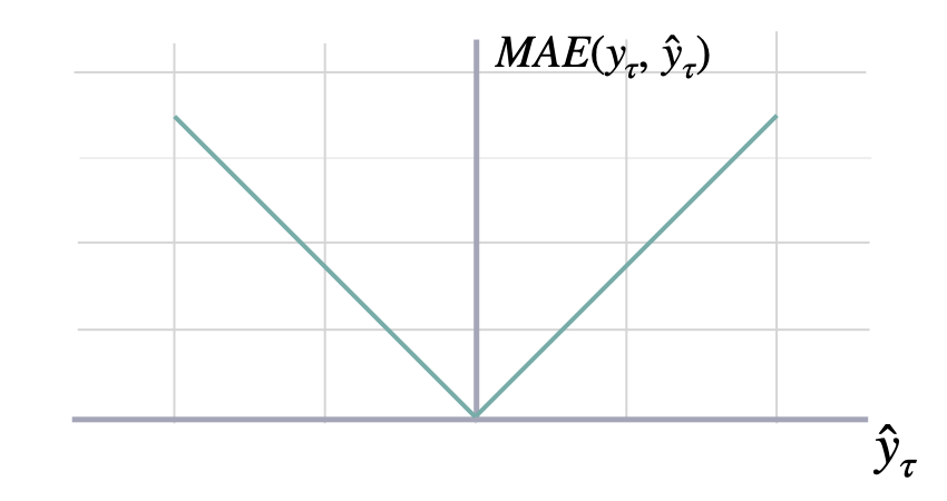
均方误差 (MSE)
class MSE(BasePointLoss):
    """  Mean Squared Error

    Calculates Mean Squared Error between
    `y` and `y_hat`. MSE measures the relative prediction
    accuracy of a forecasting method by calculating the
    squared deviation of the prediction and the true
    value at a given time, and averages these devations
    over the length of the series.

    $$ \mathrm{MSE}(\\mathbf{y}_{\\tau}, \\mathbf{\hat{y}}_{\\tau}) = \\frac{1}{H} \\sum^{t+H}_{\\tau=t+1} (y_{\\tau} - \hat{y}_{\\tau})^{2} $$

    **Parameters:**<br>
    `horizon_weight`: Tensor of size h, weight for each timestamp of the forecasting window. <br>
    """
    def __init__(self, horizon_weight=None):
        super(MSE, self).__init__(horizon_weight=horizon_weight,
                                  outputsize_multiplier=1,
                                  output_names=[''])

    def __call__(self,
                 y: torch.Tensor,
                 y_hat: torch.Tensor,
                 mask: Union[torch.Tensor, None] = None):
        """
        **Parameters:**<br>
        `y`: tensor, Actual values.<br>
        `y_hat`: tensor, Predicted values.<br>
        `mask`: tensor, Specifies datapoints to consider in loss.<br>

        **Returns:**<br>
        `mse`: tensor (single value).
        """
        losses = (y - y_hat)**2
        weights = self._compute_weights(y=y, mask=mask)
        return _weighted_mean(losses=losses, weights=weights)
show_doc(MSE, name='MSE.__init__', title_level=3)show_doc(MSE.__call__, name='MSE.__call__', title_level=3)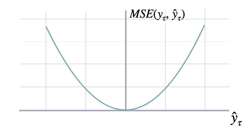
均方根误差 (RMSE)
class RMSE(BasePointLoss):
    """ Root Mean Squared Error

    Calculates Root Mean Squared Error between
    `y` and `y_hat`. RMSE measures the relative prediction
    accuracy of a forecasting method by calculating the squared deviation
    of the prediction and the observed value at a given time and
    averages these devations over the length of the series.
    Finally the RMSE will be in the same scale
    as the original time series so its comparison with other
    series is possible only if they share a common scale.
    RMSE has a direct connection to the L2 norm.

    $$ \mathrm{RMSE}(\\mathbf{y}_{\\tau}, \\mathbf{\hat{y}}_{\\tau}) = \\sqrt{\\frac{1}{H} \\sum^{t+H}_{\\tau=t+1} (y_{\\tau} - \hat{y}_{\\tau})^{2}} $$

    **Parameters:**<br>
    `horizon_weight`: Tensor of size h, weight for each timestamp of the forecasting window. <br>
    """
    def __init__(self, horizon_weight=None):
        super(RMSE, self).__init__(horizon_weight=horizon_weight,
                                  outputsize_multiplier=1,
                                  output_names=[''])

    def __call__(self,
                 y: torch.Tensor,
                 y_hat: torch.Tensor,
                 mask: Union[torch.Tensor, None] = None):
        """
        **Parameters:**<br>
        `y`: tensor, Actual values.<br>
        `y_hat`: tensor, Predicted values.<br>
        `mask`: tensor, Specifies datapoints to consider in loss.<br>

        **Returns:**<br>
        `rmse`: tensor (single value).
        """
        losses = (y - y_hat)**2
        weights = self._compute_weights(y=y, mask=mask)
        losses = _weighted_mean(losses=losses, weights=weights)
        return torch.sqrt(losses)
show_doc(RMSE, name='RMSE.__init__', title_level=3)show_doc(RMSE.__call__, name='RMSE.__call__', title_level=3)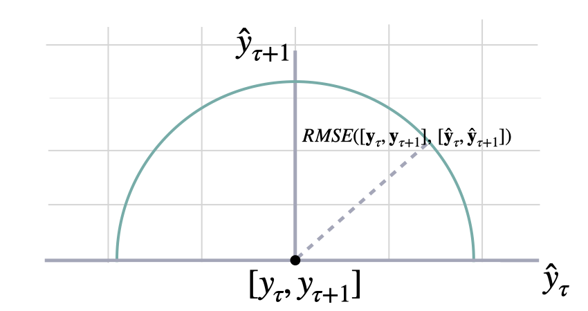
2. 百分比误差
这些指标是无单位的,适合于跨系列的比较。
平均绝对百分比误差 (MAPE)
class MAPE(BasePointLoss):
    """ Mean Absolute Percentage Error

    Calculates Mean Absolute Percentage Error  between
    `y` and `y_hat`. MAPE measures the relative prediction
    accuracy of a forecasting method by calculating the percentual deviation
    of the prediction and the observed value at a given time and
    averages these devations over the length of the series.
    The closer to zero an observed value is, the higher penalty MAPE loss
    assigns to the corresponding error.

    $$ \mathrm{MAPE}(\\mathbf{y}_{\\tau}, \\mathbf{\hat{y}}_{\\tau}) = \\frac{1}{H} \\sum^{t+H}_{\\tau=t+1} \\frac{|y_{\\tau}-\hat{y}_{\\tau}|}{|y_{\\tau}|} $$

    **Parameters:**<br>
    `horizon_weight`: Tensor of size h, weight for each timestamp of the forecasting window. <br>

    **References:**<br>
    [Makridakis S., "Accuracy measures: theoretical and practical concerns".](https://www.sciencedirect.com/science/article/pii/0169207093900793)
    """
    def __init__(self, horizon_weight=None):
        super(MAPE, self).__init__(horizon_weight=horizon_weight,
                                  outputsize_multiplier=1,
                                  output_names=[''])

    def __call__(self,
                 y: torch.Tensor,
                 y_hat: torch.Tensor,
                 mask: Union[torch.Tensor, None] = None):
        """
        **Parameters:**<br>
        `y`: tensor, Actual values.<br>
        `y_hat`: tensor, Predicted values.<br>
        `mask`: tensor, Specifies date stamps per serie to consider in loss.<br>

        **Returns:**<br>
        `mape`: tensor (single value).
        """
        scale = _divide_no_nan(torch.ones_like(y, device=y.device), torch.abs(y))
        losses = torch.abs(y - y_hat) * scale
        weights = self._compute_weights(y=y, mask=mask)
        mape = _weighted_mean(losses=losses, weights=weights)
        return mape
show_doc(MAPE, name='MAPE.__init__', title_level=3)show_doc(MAPE.__call__, name='MAPE.__call__', title_level=3)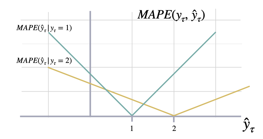
对称平均绝对百分比误差 (sMAPE)
class SMAPE(BasePointLoss):
    """ Symmetric Mean Absolute Percentage Error

    Calculates Symmetric Mean Absolute Percentage Error between
    `y` and `y_hat`. SMAPE measures the relative prediction
    accuracy of a forecasting method by calculating the relative deviation
    of the prediction and the observed value scaled by the sum of the
    absolute values for the prediction and observed value at a
    given time, then averages these devations over the length
    of the series. This allows the SMAPE to have bounds between
    0% and 200% which is desireble compared to normal MAPE that
    may be undetermined when the target is zero.

    $$ \mathrm{sMAPE}_{2}(\\mathbf{y}_{\\tau}, \\mathbf{\hat{y}}_{\\tau}) = \\frac{1}{H} \\sum^{t+H}_{\\tau=t+1} \\frac{|y_{\\tau}-\hat{y}_{\\tau}|}{|y_{\\tau}|+|\hat{y}_{\\tau}|} $$

    **Parameters:**<br>
    `horizon_weight`: Tensor of size h, weight for each timestamp of the forecasting window. <br>

    **References:**<br>
    [Makridakis S., "Accuracy measures: theoretical and practical concerns".](https://www.sciencedirect.com/science/article/pii/0169207093900793)
    """
    def __init__(self, horizon_weight=None):
        super(SMAPE, self).__init__(horizon_weight=horizon_weight,
                                  outputsize_multiplier=1,
                                  output_names=[''])

    def __call__(self,
                 y: torch.Tensor,
                 y_hat: torch.Tensor,
                 mask: Union[torch.Tensor, None] = None):
        """
        **Parameters:**<br>
        `y`: tensor, Actual values.<br>
        `y_hat`: tensor, Predicted values.<br>
        `mask`: tensor, Specifies date stamps per serie to consider in loss.<br>

        **Returns:**<br>
        `smape`: tensor (single value).
        """
        delta_y = torch.abs((y - y_hat))
        scale = torch.abs(y) + torch.abs(y_hat)
        losses = _divide_no_nan(delta_y, scale)
        weights = self._compute_weights(y=y, mask=mask)
        return 2*_weighted_mean(losses=losses, weights=weights)
show_doc(SMAPE, name='SMAPE.__init__', title_level=3)show_doc(SMAPE.__call__, name='SMAPE.__call__', title_level=3)3. 与尺度无关的误差
这些指标测量相对于基准的相对改进。
平均绝对缩放误差 (MASE)
class MASE(BasePointLoss):
    """ Mean Absolute Scaled Error
    Calculates the Mean Absolute Scaled Error between
    `y` and `y_hat`. MASE measures the relative prediction
    accuracy of a forecasting method by comparinng the mean absolute errors
    of the prediction and the observed value against the mean
    absolute errors of the seasonal naive model.
    The MASE partially composed the Overall Weighted Average (OWA),
    used in the M4 Competition.

    $$ \mathrm{MASE}(\\mathbf{y}_{\\tau}, \\mathbf{\hat{y}}_{\\tau}, \\mathbf{\hat{y}}^{season}_{\\tau}) = \\frac{1}{H} \sum^{t+H}_{\\tau=t+1} \\frac{|y_{\\tau}-\hat{y}_{\\tau}|}{\mathrm{MAE}(\\mathbf{y}_{\\tau}, \\mathbf{\hat{y}}^{season}_{\\tau})} $$

    **Parameters:**<br>
    `seasonality`: int. Main frequency of the time series; Hourly 24,  Daily 7, Weekly 52, Monthly 12, Quarterly 4, Yearly 1.
    `horizon_weight`: Tensor of size h, weight for each timestamp of the forecasting window. <br>

    **References:**<br>
    [Rob J. Hyndman, & Koehler, A. B. "Another look at measures of forecast accuracy".](https://www.sciencedirect.com/science/article/pii/S0169207006000239)<br>
    [Spyros Makridakis, Evangelos Spiliotis, Vassilios Assimakopoulos, "The M4 Competition: 100,000 time series and 61 forecasting methods".](https://www.sciencedirect.com/science/article/pii/S0169207019301128)
    """
    def __init__(self, seasonality: int, horizon_weight=None):
        super(MASE, self).__init__(horizon_weight=horizon_weight,
                                   outputsize_multiplier=1,
                                   output_names=[''])
        self.seasonality = seasonality

    def __call__(self,
                 y: torch.Tensor,
                 y_hat: torch.Tensor,
                 y_insample: torch.Tensor,
                 mask: Union[torch.Tensor, None] = None):
        """
        **Parameters:**<br>
        `y`: tensor (batch_size, output_size), Actual values.<br>
        `y_hat`: tensor (batch_size, output_size)), Predicted values.<br>
        `y_insample`: tensor (batch_size, input_size), Actual insample Seasonal Naive predictions.<br>
        `mask`: tensor, Specifies date stamps per serie to consider in loss.<br>

        **Returns:**<br>
        `mase`: tensor (single value).
        """
        delta_y = torch.abs(y - y_hat)
        scale = torch.mean(torch.abs(y_insample[:, self.seasonality:] - \
                                     y_insample[:, :-self.seasonality]), axis=1)
        losses = _divide_no_nan(delta_y, scale[:, None])
        weights = self._compute_weights(y=y, mask=mask)
        return _weighted_mean(losses=losses, weights=weights)
show_doc(MASE, name='MASE.__init__', title_level=3)show_doc(MASE.__call__, name='MASE.__call__', title_level=3)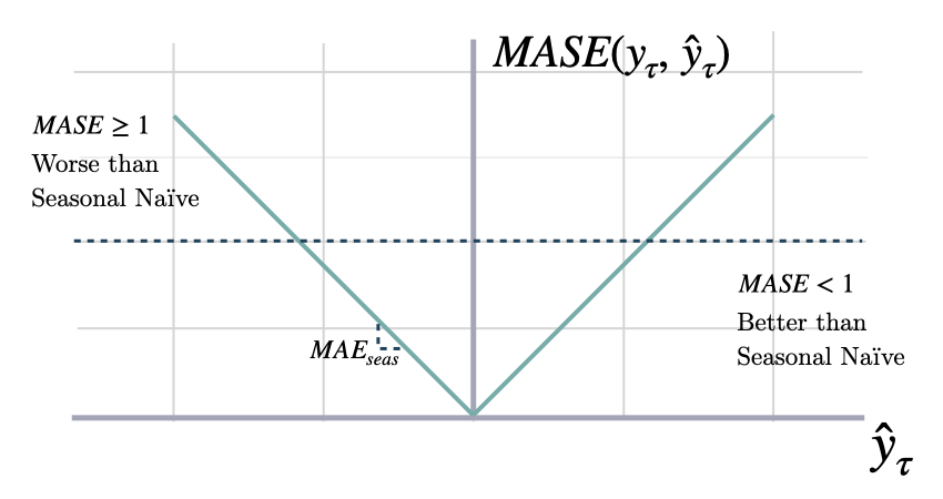
相对均方误差 (relMSE)
class relMSE(BasePointLoss):
    """Relative Mean Squared Error
    Computes Relative Mean Squared Error (relMSE), as proposed by Hyndman & Koehler (2006)
    as an alternative to percentage errors, to avoid measure unstability.
    $$ \mathrm{relMSE}(\\mathbf{y}, \\mathbf{\hat{y}}, \\mathbf{\hat{y}}^{naive1}) =
    \\frac{\mathrm{MSE}(\\mathbf{y}, \\mathbf{\hat{y}})}{\mathrm{MSE}(\\mathbf{y}, \\mathbf{\hat{y}}^{naive1})} $$

    **Parameters:**<br>
    `y_train`: numpy array, Training values.<br>
    `horizon_weight`: Tensor of size h, weight for each timestamp of the forecasting window. <br>

    **References:**<br>
    - [Hyndman, R. J and Koehler, A. B. (2006).
       "Another look at measures of forecast accuracy",
       International Journal of Forecasting, Volume 22, Issue 4.](https://www.sciencedirect.com/science/article/pii/S0169207006000239)<br>
    - [Kin G. Olivares, O. Nganba Meetei, Ruijun Ma, Rohan Reddy, Mengfei Cao, Lee Dicker.
       "Probabilistic Hierarchical Forecasting with Deep Poisson Mixtures.
       Submitted to the International Journal Forecasting, Working paper available at arxiv.](https://arxiv.org/pdf/2110.13179.pdf)
    """
    def __init__(self, y_train, horizon_weight=None):
        super(relMSE, self).__init__(horizon_weight=horizon_weight,
                                     outputsize_multiplier=1,
                                     output_names=[''])
        self.y_train = y_train
        self.mse = MSE(horizon_weight=horizon_weight)

    def __call__(self,
                 y: torch.Tensor,
                 y_hat: torch.Tensor,
                 mask: Union[torch.Tensor, None] = None):
        """
        **Parameters:**<br>
        `y`: tensor (batch_size, output_size), Actual values.<br>
        `y_hat`: tensor (batch_size, output_size)), Predicted values.<br>
        `y_insample`: tensor (batch_size, input_size), Actual insample Seasonal Naive predictions.<br>
        `mask`: tensor, Specifies date stamps per serie to consider in loss.<br>

        **Returns:**<br>
        `relMSE`: tensor (single value).
        """
        horizon = y.shape[-1]
        last_col = self.y_train[:, -1].unsqueeze(1)
        y_naive = last_col.repeat(1, horizon)

        norm = self.mse(y=y, y_hat=y_naive, mask=mask) # 已经加权
        norm = norm + 1e-5 # 数值稳定性
        loss = self.mse(y=y, y_hat=y_hat, mask=mask) # 已经加权
        loss = _divide_no_nan(loss, norm)
        return loss
show_doc(relMSE, name='relMSE.__init__', title_level=3)show_doc(relMSE.__call__, name='relMSE.__call__', title_level=3)4. 概率错误
这些方法使用统计方法通过观察到的数据来估计未知的概率分布。
最大似然估计涉及找到最大化似然函数的参数值,似然函数衡量的是在给定参数值的情况下获得观察到的数据的概率。最大似然估计在满足某些假设时具有良好的理论性质和效率。
在非参数方法中,分位数回归测量不对称偏差,产生低估/高估。
分位损失
class QuantileLoss(BasePointLoss):
    """ Quantile Loss

    Computes the quantile loss between `y` and `y_hat`.
    QL measures the deviation of a quantile forecast.
    By weighting the absolute deviation in a non symmetric way, the
    loss pays more attention to under or over estimation.
    A common value for q is 0.5 for the deviation from the median (Pinball loss).

    $$ \mathrm{QL}(\\mathbf{y}_{\\tau}, \\mathbf{\hat{y}}^{(q)}_{\\tau}) = \\frac{1}{H} \\sum^{t+H}_{\\tau=t+1} \Big( (1-q)\,( \hat{y}^{(q)}_{\\tau} - y_{\\tau} )_{+} + q\,( y_{\\tau} - \hat{y}^{(q)}_{\\tau} )_{+} \Big) $$

    **Parameters:**<br>
    `q`: float, between 0 and 1. The slope of the quantile loss, in the context of quantile regression, the q determines the conditional quantile level.<br>
    `horizon_weight`: Tensor of size h, weight for each timestamp of the forecasting window. <br>

    **References:**<br>
    [Roger Koenker and Gilbert Bassett, Jr., "Regression Quantiles".](https://www.jstor.org/stable/1913643)
    """
    def __init__(self, q, horizon_weight=None):
        super(QuantileLoss, self).__init__(horizon_weight=horizon_weight,
                                           outputsize_multiplier=1,
                                           output_names=[f'_ql{q}'])
        self.q = q

    def __call__(self,
                 y: torch.Tensor,
                 y_hat: torch.Tensor,
                 mask: Union[torch.Tensor, None] = None):
        """
        **Parameters:**<br>
        `y`: tensor, Actual values.<br>
        `y_hat`: tensor, Predicted values.<br>
        `mask`: tensor, Specifies datapoints to consider in loss.<br>

        **Returns:**<br>
        `quantile_loss`: tensor (single value).
        """
        delta_y = y - y_hat
        losses = torch.max(torch.mul(self.q, delta_y), torch.mul((self.q - 1), delta_y))
        weights = self._compute_weights(y=y, mask=mask)
        return _weighted_mean(losses=losses, weights=weights)
show_doc(QuantileLoss, name='QuantileLoss.__init__', title_level=3)show_doc(QuantileLoss.__call__, name='QuantileLoss.__call__', title_level=3)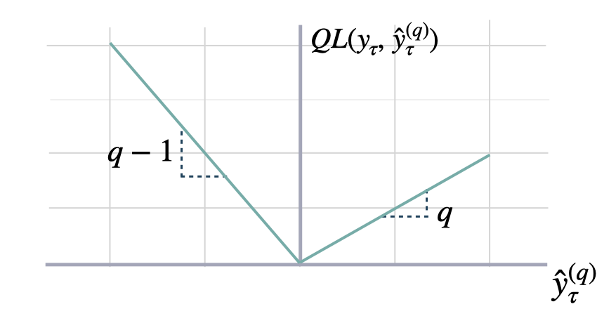
多量化损失(MQLoss)
def level_to_outputs(level):
    qs = sum([[50-l/2, 50+l/2] for l in level], [])
    output_names = sum([[f'-lo-{l}', f'-hi-{l}'] for l in level], [])

    sort_idx = np.argsort(qs)
    quantiles = np.array(qs)[sort_idx]

    # 添加默认中位数
    quantiles = np.concatenate([np.array([50]), quantiles])
    quantiles = torch.Tensor(quantiles) / 100
    output_names = list(np.array(output_names)[sort_idx])
    output_names.insert(0, '-median')

    return quantiles, output_names

def quantiles_to_outputs(quantiles):
    output_names = []
    for q in quantiles:
        if q<.50:
            output_names.append(f'-lo-{np.round(100-200*q,2)}')
        elif q>.50:
            output_names.append(f'-hi-{np.round(100-200*(1-q),2)}')
        else:
            output_names.append('-median')
    return quantiles, output_names
class MQLoss(BasePointLoss):
""" Multi-Quantile loss
Calculates the Multi-Quantile loss (MQL) between `y` and `y_hat`.
MQL calculates the average multi-quantile Loss for
a given set of quantiles, based on the absolute
difference between predicted quantiles and observed values.
$$ \mathrm{MQL}(\\mathbf{y}_{\\tau},[\\mathbf{\hat{y}}^{(q_{1})}_{\\tau}, ... ,\hat{y}^{(q_{n})}_{\\tau}]) = \\frac{1}{n} \\sum_{q_{i}} \mathrm{QL}(\\mathbf{y}_{\\tau}, \\mathbf{\hat{y}}^{(q_{i})}_{\\tau}) $$
The limit behavior of MQL allows to measure the accuracy
of a full predictive distribution $\mathbf{\hat{F}}_{\\tau}$ with
the continuous ranked probability score (CRPS). This can be achieved
through a numerical integration technique, that discretizes the quantiles
and treats the CRPS integral with a left Riemann approximation, averaging over
uniformly distanced quantiles.
$$ \mathrm{CRPS}(y_{\\tau}, \mathbf{\hat{F}}_{\\tau}) = \int^{1}_{0} \mathrm{QL}(y_{\\tau}, \hat{y}^{(q)}_{\\tau}) dq $$
**Parameters:**<br>
`level`: int list [0,100]. Probability levels for prediction intervals (Defaults median).
`quantiles`: float list [0., 1.]. Alternative to level, quantiles to estimate from y distribution.
`horizon_weight`: Tensor of size h, weight for each timestamp of the forecasting window. <br>
**References:**<br>
[Roger Koenker and Gilbert Bassett, Jr., "Regression Quantiles".](https://www.jstor.org/stable/1913643)<br>
[James E. Matheson and Robert L. Winkler, "Scoring Rules for Continuous Probability Distributions".](https://www.jstor.org/stable/2629907)
"""
def __init__(self, level=[80, 90], quantiles=None, horizon_weight=None):
qs, output_names = level_to_outputs(level)
qs = torch.Tensor(qs)
# 将分位数转换为同质输出名称
if quantiles is not None:
_, output_names = quantiles_to_outputs(quantiles)
qs = torch.Tensor(quantiles)
super(MQLoss, self).__init__(horizon_weight=horizon_weight,
outputsize_multiplier=len(qs),
output_names=output_names)
self.quantiles = torch.nn.Parameter(qs, requires_grad=False)
def domain_map(self, y_hat: torch.Tensor):
"""
身份域映射 [B,T,H,Q]/[B,H,Q]
"""
return y_hat
def _compute_weights(self, y, mask):
"""
Compute final weights for each datapoint (based on all weights and all masks)
Set horizon_weight to a ones[H] tensor if not set.
If set, check that it has the same length as the horizon in x.
"""
if mask is None:
mask = torch.ones_like(y, device=y.device)
else:
mask = mask.unsqueeze(1) # 添加Q维度。
if self.horizon_weight is None:
self.horizon_weight = torch.ones(mask.shape[-1])
else:
assert mask.shape[-1] == len(self.horizon_weight), \
'horizon_weight must have same length as Y'
weights = self.horizon_weight.clone()
weights = torch.ones_like(mask, device=mask.device) * weights.to(mask.device)
return weights * mask
def __call__(self,
y: torch.Tensor,
y_hat: torch.Tensor,
mask: Union[torch.Tensor, None] = None):
"""
**Parameters:**<br>
`y`: tensor, Actual values.<br>
`y_hat`: tensor, Predicted values.<br>
`mask`: tensor, Specifies date stamps per serie to consider in loss.<br>
**Returns:**<br>
`mqloss`: tensor (single value).
"""
error = y_hat - y.unsqueeze(-1)
sq = torch.maximum(-error, torch.zeros_like(error))
s1_q = torch.maximum(error, torch.zeros_like(error))
losses = (1/len(self.quantiles))*(self.quantiles * sq + (1 - self.quantiles) * s1_q)
if y_hat.ndim == 3: # 基础窗口
losses = losses.swapaxes(-2,-1) # [B,H,Q] -> [B,Q,H](用于水平加权,H置于末尾)
elif y_hat.ndim == 4: # 基础循环
losses = losses.swapaxes(-2,-1)
losses = losses.swapaxes(-2,-3) # [B,seq_len,H,Q] -> [B,Q,seq_len,H] (用于水平加权,H置于末尾)
weights = self._compute_weights(y=losses, mask=mask) # 利用损失增加暗度
# 注意:权重没有Q维度。
return _weighted_mean(losses=losses, weights=weights)show_doc(MQLoss, name='MQLoss.__init__', title_level=3)show_doc(MQLoss.__call__, name='MQLoss.__call__', title_level=3)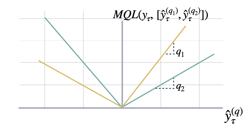
::: {#da37f2ef .cell 0=‘隐’ 1=‘藏’}
# 单元测试以检查 MQLoss 存储的分位数
# 属性已正确实例化
check = MQLoss(level=[80, 90])
test_eq(len(check.quantiles), 5)

check = MQLoss(quantiles=[0.0100, 0.1000, 0.5, 0.9000, 0.9900])
print(check.output_names)
print(check.quantiles)
test_eq(len(check.quantiles), 5)

check = MQLoss(quantiles=[0.0100, 0.1000, 0.9000, 0.9900])
test_eq(len(check.quantiles), 4)
:::
隐式分位数损失(IQLoss)
class QuantileLayer(nn.Module):
    r"""
    Implicit Quantile Layer from the paper ``IQN for Distributional
    Reinforcement Learning`` (https://arxiv.org/abs/1806.06923) by
    Dabney et al. 2018.

    Code from GluonTS: https://github.com/awslabs/gluonts/blob/61133ef6e2d88177b32ace4afc6843ab9a7bc8cd/src/gluonts/torch/distributions/implicit_quantile_network.py

    """

    def __init__(self, num_output: int, cos_embedding_dim: int = 128):
        super().__init__()

        self.output_layer = nn.Sequential(
            nn.Linear(cos_embedding_dim, cos_embedding_dim),
            nn.PReLU(),
            nn.Linear(cos_embedding_dim, num_output),
        )

        self.register_buffer("integers", torch.arange(0, cos_embedding_dim))

    def forward(self, tau: torch.Tensor) -> torch.Tensor:
        cos_emb_tau = torch.cos(tau * self.integers * torch.pi)
        return self.output_layer(cos_emb_tau)


class IQLoss(QuantileLoss):
    """Implicit Quantile Loss

    Computes the quantile loss between `y` and `y_hat`, with the quantile `q` provided as an input to the network.
    IQL measures the deviation of a quantile forecast.
    By weighting the absolute deviation in a non symmetric way, the
    loss pays more attention to under or over estimation.

    $$ \mathrm{QL}(\\mathbf{y}_{\\tau}, \\mathbf{\hat{y}}^{(q)}_{\\tau}) = \\frac{1}{H} \\sum^{t+H}_{\\tau=t+1} \Big( (1-q)\,( \hat{y}^{(q)}_{\\tau} - y_{\\tau} )_{+} + q\,( y_{\\tau} - \hat{y}^{(q)}_{\\tau} )_{+} \Big) $$

    **Parameters:**<br>
    `quantile_sampling`: str, default='uniform', sampling distribution used to sample the quantiles during training. Choose from ['uniform', 'beta']. <br>
    `horizon_weight`: Tensor of size h, weight for each timestamp of the forecasting window. <br>

    **References:**<br>
    [Gouttes, Adèle, Kashif Rasul, Mateusz Koren, Johannes Stephan, and Tofigh Naghibi, "Probabilistic Time Series Forecasting with Implicit Quantile Networks".](http://arxiv.org/abs/2107.03743)
    """
    def __init__(self, cos_embedding_dim = 64, concentration0 = 1.0, concentration1 = 1.0, horizon_weight=None):
        self.update_quantile()
        super(IQLoss, self).__init__(
            q = self.q,
            horizon_weight=horizon_weight
        )

        self.cos_embedding_dim = cos_embedding_dim
        self.concentration0 = concentration0
        self.concentration1 = concentration1
        self.has_sampled = False
        self.has_predicted = False

        self.quantile_layer = QuantileLayer(
            num_output=1, cos_embedding_dim=self.cos_embedding_dim
        )
        self.output_layer = nn.Sequential(
            nn.Linear(1, 1), nn.PReLU()
        )

    def _sample_quantiles(self, sample_size, device):
        if not self.has_sampled:
            self._init_sampling_distribution(device)

        quantiles = self.sampling_distr.sample(sample_size)
        self.has_sampled = True
        self.has_predicted = False

        return quantiles

    def _init_sampling_distribution(self, device):
        concentration0 = torch.tensor([self.concentration0],
                                      device=device,
                                      dtype=torch.float32)
        concentration1 = torch.tensor([self.concentration1],
                                      device=device,
                                      dtype=torch.float32)
        self.sampling_distr = Beta(concentration0 = concentration0,
                                   concentration1 = concentration1)

    def update_quantile(self, q: float = 0.5):
        self.q = q
        self.output_names = [f"_ql{q}"]
        self.has_predicted = True

    def domain_map(self, y_hat):
        """
        Adds IQN network to output of network

        Input shapes to this function:

        base_windows: y_hat = [B, h, 1]
        base_multivariate: y_hat = [B, h, n_series]
        base_recurrent: y_hat = [B, seq_len, h, n_series]
        """
        if self.eval() and self.has_predicted:
            quantiles = torch.full(size=y_hat.shape,
                                    fill_value=self.q,
                                    device=y_hat.device,
                                    dtype=y_hat.dtype)
            quantiles = quantiles.unsqueeze(-1)
        else:
            quantiles = self._sample_quantiles(sample_size=y_hat.shape,
                                        device=y_hat.device)

        # 嵌入分位数并添加到 y_hat
        emb_taus = self.quantile_layer(quantiles)
        emb_inputs = y_hat.unsqueeze(-1) * (1.0 + emb_taus)
        emb_outputs = self.output_layer(emb_inputs)

        # 域图
        y_hat = emb_outputs.squeeze(-1).squeeze(-1)

        return y_hat
show_doc(IQLoss, name='IQLoss.__init__', title_level=3)show_doc(IQLoss.__call__, name='IQLoss.__call__', title_level=3)::: {#cee2992b .cell 0=‘隐’ 1=‘藏’}
# 单元测试
# 检查默认分位数在初始化时是否设置为0.5
check = IQLoss()
test_eq(check.q, 0.5)

# 检查分位数是否正确更新 - 预测
check = IQLoss()
check.update_quantile(0.7)
test_eq(check.q, 0.7)
:::
分布损失
def weighted_average(x: torch.Tensor,
                     weights: Optional[torch.Tensor]=None, dim=None) -> torch.Tensor:
    """
    Computes the weighted average of a given tensor across a given dim, masking
    values associated with weight zero,
    meaning instead of `nan * 0 = nan` you will get `0 * 0 = 0`.

    **Parameters:**<br>
    `x`: Input tensor, of which the average must be computed.<br>
    `weights`: Weights tensor, of the same shape as `x`.<br>
    `dim`: The dim along which to average `x`.<br>

    **Returns:**<br>
    `Tensor`: The tensor with values averaged along the specified `dim`.<br>
    """
    if weights is not None:
        weighted_tensor = torch.where(
            weights != 0, x * weights, torch.zeros_like(x)
        )
        sum_weights = torch.clamp(
            weights.sum(dim=dim) if dim else weights.sum(), min=1.0
        )
        return (
            weighted_tensor.sum(dim=dim) if dim else weighted_tensor.sum()
        ) / sum_weights
    else:
        return x.mean(dim=dim)
def bernoulli_domain_map(input: torch.Tensor):
""" Bernoulli Domain Map
Maps input into distribution constraints, by construction input's
last dimension is of matching `distr_args` length.
**Parameters:**<br>
`input`: tensor, of dimensions [B,T,H,theta] or [B,H,theta].<br>
**Returns:**<br>
`(probs,)`: tuple with tensors of Poisson distribution arguments.<br>
"""
return (input.squeeze(-1),)
def bernoulli_scale_decouple(output, loc=None, scale=None):
""" Bernoulli Scale Decouple
Stabilizes model's output optimization, by learning residual
variance and residual location based on anchoring `loc`, `scale`.
Also adds Bernoulli domain protection to the distribution parameters.
"""
probs = output[0]
#如果(位置不为空)且(尺度不为空):
# 速率 = (速率 * 比例) + 位置
probs = F.sigmoid(probs)#.clone()
return (probs,)
def student_domain_map(input: torch.Tensor):
""" Student T Domain Map
Maps input into distribution constraints, by construction input's
last dimension is of matching `distr_args` length.
**Parameters:**<br>
`input`: tensor, of dimensions [B,T,H,theta] or [B,H,theta].<br>
`eps`: float, helps the initialization of scale for easier optimization.<br>
**Returns:**<br>
`(df, loc, scale)`: tuple with tensors of StudentT distribution arguments.<br>
"""
df, loc, scale = torch.tensor_split(input, 3, dim=-1)
return df.squeeze(-1), loc.squeeze(-1), scale.squeeze(-1)
def student_scale_decouple(output, loc=None, scale=None, eps: float=0.1):
""" Normal Scale Decouple
Stabilizes model's output optimization, by learning residual
variance and residual location based on anchoring `loc`, `scale`.
Also adds StudentT domain protection to the distribution parameters.
"""
df, mean, tscale = output
tscale = F.softplus(tscale)
if (loc is not None) and (scale is not None):
mean = (mean * scale) + loc
tscale = (tscale + eps) * scale
df = 2.0 + F.softplus(df)
return (df, mean, tscale)
def normal_domain_map(input: torch.Tensor):
""" Normal Domain Map
Maps input into distribution constraints, by construction input's
last dimension is of matching `distr_args` length.
**Parameters:**<br>
`input`: tensor, of dimensions [B,T,H,theta] or [B,H,theta].<br>
`eps`: float, helps the initialization of scale for easier optimization.<br>
**Returns:**<br>
`(mean, std)`: tuple with tensors of Normal distribution arguments.<br>
"""
mean, std = torch.tensor_split(input, 2, dim=-1)
return mean.squeeze(-1), std.squeeze(-1)
def normal_scale_decouple(output, loc=None, scale=None, eps: float=0.2):
""" Normal Scale Decouple
Stabilizes model's output optimization, by learning residual
variance and residual location based on anchoring `loc`, `scale`.
Also adds Normal domain protection to the distribution parameters.
"""
mean, std = output
std = F.softplus(std)
if (loc is not None) and (scale is not None):
mean = (mean * scale) + loc
std = (std + eps) * scale
return (mean, std)
def poisson_domain_map(input: torch.Tensor):
""" Poisson Domain Map
Maps input into distribution constraints, by construction input's
last dimension is of matching `distr_args` length.
**Parameters:**<br>
`input`: tensor, of dimensions [B,T,H,theta] or [B,H,theta].<br>
**Returns:**<br>
`(rate,)`: tuple with tensors of Poisson distribution arguments.<br>
"""
return (input.squeeze(-1),)
def poisson_scale_decouple(output, loc=None, scale=None):
""" Poisson Scale Decouple
Stabilizes model's output optimization, by learning residual
variance and residual location based on anchoring `loc`, `scale`.
Also adds Poisson domain protection to the distribution parameters.
"""
eps = 1e-10
rate = output[0]
if (loc is not None) and (scale is not None):
rate = (rate * scale) + loc
rate = F.softplus(rate) + eps
return (rate,)
def nbinomial_domain_map(input: torch.Tensor):
""" Negative Binomial Domain Map
Maps input into distribution constraints, by construction input's
last dimension is of matching `distr_args` length.
**Parameters:**<br>
`input`: tensor, of dimensions [B,T,H,theta] or [B,H,theta].<br>
**Returns:**<br>
`(total_count, alpha)`: tuple with tensors of N.Binomial distribution arguments.<br>
"""
mu, alpha = torch.tensor_split(input, 2, dim=-1)
return mu.squeeze(-1), alpha.squeeze(-1)
def nbinomial_scale_decouple(output, loc=None, scale=None):
""" Negative Binomial Scale Decouple
Stabilizes model's output optimization, by learning total
count and logits based on anchoring `loc`, `scale`.
Also adds Negative Binomial domain protection to the distribution parameters.
"""
mu, alpha = output
mu = F.softplus(mu) + 1e-8
alpha = F.softplus(alpha) + 1e-8 # alpha = 1 / 总计数
if (loc is not None) and (scale is not None):
mu *= loc
alpha /= (loc + 1.)
# mu = 总数量 * (概率/(1-概率))
# => 概率 = μ / (总计数 + μ)
# => 概率 = mu / [总次数 * (1 + mu * (1/总次数))]
total_count = 1.0 / alpha
probs = (mu * alpha / (1.0 + mu * alpha)) + 1e-8
return (total_count, probs)def est_lambda(mu, rho):
return mu ** (2 - rho) / (2 - rho)
def est_alpha(rho):
return (2 - rho) / (rho - 1)
def est_beta(mu, rho):
return mu ** (1 - rho) / (rho - 1)
class Tweedie(Distribution):
""" Tweedie Distribution
The Tweedie distribution is a compound probability, special case of exponential
dispersion models EDMs defined by its mean-variance relationship.
The distribution particularly useful to model sparse series as the probability has
possitive mass at zero but otherwise is continuous.
$Y \sim \mathrm{ED}(\\mu,\\sigma^{2}) \qquad
\mathbb{P}(y|\\mu ,\\sigma^{2})=h(\\sigma^{2},y) \\exp \\left({\\frac {\\theta y-A(\\theta )}{\\sigma^{2}}}\\right)$<br>
$\mu =A'(\\theta ) \qquad \mathrm{Var}(Y) = \\sigma^{2} \\mu^{\\rho}$
Cases of the variance relationship include Normal (`rho` = 0), Poisson (`rho` = 1),
Gamma (`rho` = 2), inverse Gaussian (`rho` = 3).
**Parameters:**<br>
`log_mu`: tensor, with log of means.<br>
`rho`: float, Tweedie variance power (1,2). Fixed across all observations.<br>
`sigma2`: tensor, Tweedie variance. Currently fixed in 1.<br>
**References:**<br>
- [Tweedie, M. C. K. (1984). An index which distinguishes between some important exponential families. Statistics: Applications and New Directions.
Proceedings of the Indian Statistical Institute Golden Jubilee International Conference (Eds. J. K. Ghosh and J. Roy), pp. 579-604. Calcutta: Indian Statistical Institute.]()<br>
- [Jorgensen, B. (1987). Exponential Dispersion Models. Journal of the Royal Statistical Society.
Series B (Methodological), 49(2), 127–162. http://www.jstor.org/stable/2345415](http://www.jstor.org/stable/2345415)<br>
"""
def __init__(self, log_mu, rho, validate_args=None):
# TODO: add sigma2 dispersion
# TODO add constraints
# arg_constraints = {'log_mu': constraints.real, 'rho': constraints.positive}
# support = constraints.real
self.log_mu = log_mu
self.rho = rho
assert rho>1 and rho<2, f'rho={rho} parameter needs to be between (1,2).'
batch_shape = log_mu.size()
super(Tweedie, self).__init__(batch_shape, validate_args=validate_args)
@property
def mean(self):
return torch.exp(self.log_mu)
@property
def variance(self):
return torch.ones_line(self.log_mu) #TODO need to be assigned
def sample(self, sample_shape=torch.Size()):
shape = self._extended_shape(sample_shape)
with torch.no_grad():
mu = self.mean
rho = self.rho * torch.ones_like(mu)
sigma2 = 1 #TODO
rate = est_lambda(mu, rho) / sigma2 # rate for poisson
alpha = est_alpha(rho) # alpha for Gamma distribution
beta = est_beta(mu, rho) / sigma2 # beta for Gamma distribution
# Expand for sample
rate = rate.expand(shape)
alpha = alpha.expand(shape)
beta = beta.expand(shape)
N = torch.poisson(rate)
gamma = torch.distributions.gamma.Gamma(N*alpha, beta)
samples = gamma.sample()
samples[N==0] = 0
return samples
def log_prob(self, y_true):
rho = self.rho
y_pred = self.log_mu
a = y_true * torch.exp((1 - rho) * y_pred) / (1 - rho)
b = torch.exp((2 - rho) * y_pred) / (2 - rho)
return a - b
def tweedie_domain_map(input: torch.Tensor):
""" Tweedie Domain Map
Maps input into distribution constraints, by construction input's
last dimension is of matching `distr_args` length.
**Parameters:**<br>
`input`: tensor, of dimensions [B,T,H,theta] or [B,H,theta].<br>
**Returns:**<br>
`(log_mu,)`: tuple with tensors of Tweedie distribution arguments.<br>
"""
# log_mu, probs = torch.tensor_split(input, 2, dim=-1)
return (input.squeeze(-1),)
def tweedie_scale_decouple(output, loc=None, scale=None):
""" Tweedie Scale Decouple
Stabilizes model's output optimization, by learning total
count and logits based on anchoring `loc`, `scale`.
Also adds Tweedie domain protection to the distribution parameters.
"""
log_mu = output[0]
if (loc is not None) and (scale is not None):
log_mu += torch.log(loc) # 待办事项:ρ 缩放
return (log_mu,)# 代码改编自:https://github.com/awslabs/gluonts/blob/61133ef6e2d88177b32ace4afc6843ab9a7bc8cd/src/gluonts/torch/distributions/isqf.py
class ISQF(TransformedDistribution):
"""
Distribution class for the Incremental (Spline) Quantile Function.
**Parameters:**<br>
`spline_knots`: Tensor parametrizing the x-positions of the spline knots. Shape: (*batch_shape, (num_qk-1), num_pieces)
`spline_heights`: Tensor parametrizing the y-positions of the spline knots. Shape: (*batch_shape, (num_qk-1), num_pieces)
`beta_l`: Tensor containing the non-negative learnable parameter of the left tail. Shape: (*batch_shape,)
`beta_r`: Tensor containing the non-negative learnable parameter of the right tail. Shape: (*batch_shape,)
`qk_y`: Tensor containing the increasing y-positions of the quantile knots. Shape: (*batch_shape, num_qk)
`qk_x`: Tensor containing the increasing x-positions of the quantile knots. Shape: (*batch_shape, num_qk)
`loc`: Tensor containing the location in case of a transformed random variable. Shape: (*batch_shape,)
`scale`: Tensor containing the scale in case of a transformed random variable. Shape: (*batch_shape,)
**References:**<br>
[Park, Youngsuk, Danielle Maddix, François-Xavier Aubet, Kelvin Kan, Jan Gasthaus, and Yuyang Wang (2022). "Learning Quantile Functions without Quantile Crossing for Distribution-free Time Series Forecasting".](https://proceedings.mlr.press/v151/park22a.html)
"""
def __init__(
self,
spline_knots: torch.Tensor,
spline_heights: torch.Tensor,
beta_l: torch.Tensor,
beta_r: torch.Tensor,
qk_y: torch.Tensor,
qk_x: torch.Tensor,
loc: torch.Tensor,
scale: torch.Tensor,
validate_args=None,
) -> None:
base_distribution = BaseISQF(spline_knots=spline_knots,
spline_heights=spline_heights,
beta_l=beta_l,
beta_r=beta_r,
qk_y=qk_y,
qk_x=qk_x,
validate_args=validate_args)
transforms = AffineTransform(loc = loc, scale = scale)
super().__init__(
base_distribution, transforms, validate_args=validate_args
)
def crps(self, y: torch.Tensor) -> torch.Tensor:
z = y
scale = 1.0
t = self.transforms[0]
z = t._inverse(z)
scale *= t.scale
p = self.base_dist.crps(z)
return p * scale
class BaseISQF(Distribution):
"""
Base distribution class for the Incremental (Spline) Quantile Function.
**Parameters:**<br>
`spline_knots`: Tensor parametrizing the x-positions of the spline knots. Shape: (*batch_shape, (num_qk-1), num_pieces)
`spline_heights`: Tensor parametrizing the y-positions of the spline knots. Shape: (*batch_shape, (num_qk-1), num_pieces)
`beta_l`: Tensor containing the non-negative learnable parameter of the left tail. (*batch_shape,)
`beta_r`: Tensor containing the non-negative learnable parameter of the right tail. (*batch_shape,)
`qk_y`: Tensor containing the increasing y-positions of the quantile knots. Shape: (*batch_shape, num_qk)
`qk_x`: Tensor containing the increasing x-positions of the quantile knots. Shape: (*batch_shape, num_qk)
**References:**<br>
[Park, Youngsuk, Danielle Maddix, François-Xavier Aubet, Kelvin Kan, Jan Gasthaus, and Yuyang Wang (2022). "Learning Quantile Functions without Quantile Crossing for Distribution-free Time Series Forecasting".](https://proceedings.mlr.press/v151/park22a.html)
"""
def __init__(
self,
spline_knots: torch.Tensor,
spline_heights: torch.Tensor,
beta_l: torch.Tensor,
beta_r: torch.Tensor,
qk_y: torch.Tensor,
qk_x: torch.Tensor,
tol: float = 1e-4,
validate_args: bool = False,
) -> None:
self.num_qk, self.num_pieces = qk_y.shape[-1], spline_knots.shape[-1]
self.spline_knots, self.spline_heights = spline_knots, spline_heights
self.beta_l, self.beta_r = beta_l, beta_r
self.qk_y_all = qk_y
self.tol = tol
super().__init__(
batch_shape=self.batch_shape, validate_args=validate_args
)
# 获取分位数节点(qk)参数
(
self.qk_x,
self.qk_x_plus,
self.qk_x_l,
self.qk_x_r,
) = BaseISQF.parameterize_qk(qk_x)
(
self.qk_y,
self.qk_y_plus,
self.qk_y_l,
self.qk_y_r,
) = BaseISQF.parameterize_qk(qk_y)
# 获取样条结点(sk)参数
self.sk_y, self.delta_sk_y = BaseISQF.parameterize_spline(
self.spline_heights,
self.qk_y,
self.qk_y_plus,
self.tol,
)
self.sk_x, self.delta_sk_x = BaseISQF.parameterize_spline(
self.spline_knots,
self.qk_x,
self.qk_x_plus,
self.tol,
)
if self.num_pieces > 1:
self.sk_x_plus = torch.cat(
[self.sk_x[..., 1:], self.qk_x_plus.unsqueeze(dim=-1)], dim=-1
)
else:
self.sk_x_plus = self.qk_x_plus.unsqueeze(dim=-1)
# 获取尾部参数
self.tail_al, self.tail_bl = BaseISQF.parameterize_tail(
self.beta_l, self.qk_x_l, self.qk_y_l
)
self.tail_ar, self.tail_br = BaseISQF.parameterize_tail(
-self.beta_r, 1 - self.qk_x_r, self.qk_y_r
)
@staticmethod
def parameterize_qk(
quantile_knots: torch.Tensor,
) -> Tuple[torch.Tensor, torch.Tensor, torch.Tensor, torch.Tensor]:
r"""
Function to parameterize the x or y positions
of the num_qk quantile knots
Parameters
----------
quantile_knots
x or y positions of the quantile knots
shape: (*batch_shape, num_qk)
Returns
-------
qk
x or y positions of the quantile knots (qk),
with index=1, ..., num_qk-1,
shape: (*batch_shape, num_qk-1)
qk_plus
x or y positions of the quantile knots (qk),
with index=2, ..., num_qk,
shape: (*batch_shape, num_qk-1)
qk_l
x or y positions of the left-most quantile knot (qk),
shape: (*batch_shape)
qk_r
x or y positions of the right-most quantile knot (qk),
shape: (*batch_shape)
"""
qk, qk_plus = quantile_knots[..., :-1], quantile_knots[..., 1:]
qk_l, qk_r = quantile_knots[..., 0], quantile_knots[..., -1]
return qk, qk_plus, qk_l, qk_r
@staticmethod
def parameterize_spline(
spline_knots: torch.Tensor,
qk: torch.Tensor,
qk_plus: torch.Tensor,
tol: float = 1e-4,
) -> Tuple[torch.Tensor, torch.Tensor]:
r"""
Function to parameterize the x or y positions of the spline knots
Parameters
----------
spline_knots
variable that parameterizes the spline knot positions
qk
x or y positions of the quantile knots (qk),
with index=1, ..., num_qk-1,
shape: (*batch_shape, num_qk-1)
qk_plus
x or y positions of the quantile knots (qk),
with index=2, ..., num_qk,
shape: (*batch_shape, num_qk-1)
num_pieces
number of spline knot pieces
tol
tolerance hyperparameter for numerical stability
Returns
-------
sk
x or y positions of the spline knots (sk),
shape: (*batch_shape, num_qk-1, num_pieces)
delta_sk
difference of x or y positions of the spline knots (sk),
shape: (*batch_shape, num_qk-1, num_pieces)
"""
# 样条节点之间的间距是参数化的
# 通过softmax函数(取值范围在[0,1]且总和为1)
# 我们在计算样条CRPS中的1/spacing时添加tol以防止溢出
# 添加tol后,进行归一化处理。
# (1 + num_pieces * tol)以保持总和为1的特性
num_pieces = spline_knots.shape[-1]
delta_x = (F.softmax(spline_knots, dim=-1) + tol) / (
1 + num_pieces * tol
)
zero_tensor = torch.zeros_like(
delta_x[..., 0:1]
) # 0:1 表示保持尺寸
x = torch.cat(
[zero_tensor, torch.cumsum(delta_x, dim=-1)[..., :-1]], dim=-1
)
qk, qk_plus = qk.unsqueeze(dim=-1), qk_plus.unsqueeze(dim=-1)
sk = x * (qk_plus - qk) + qk
delta_sk = delta_x * (qk_plus - qk)
return sk, delta_sk
@staticmethod
def parameterize_tail(
beta: torch.Tensor, qk_x: torch.Tensor, qk_y: torch.Tensor
) -> Tuple[torch.Tensor, torch.Tensor]:
r"""
Function to parameterize the tail parameters
Note that the exponential tails are given by
q(alpha)
= a_l log(alpha) + b_l if left tail
= a_r log(1-alpha) + b_r if right tail
where
a_l=1/beta_l, b_l=-a_l*log(qk_x_l)+q(qk_x_l)
a_r=1/beta_r, b_r=a_r*log(1-qk_x_r)+q(qk_x_r)
Parameters
----------
beta
parameterizes the left or right tail, shape: (*batch_shape,)
qk_x
left- or right-most x-positions of the quantile knots,
shape: (*batch_shape,)
qk_y
left- or right-most y-positions of the quantile knots,
shape: (*batch_shape,)
Returns
-------
tail_a
a_l or a_r as described above
tail_b
b_l or b_r as described above
"""
tail_a = 1 / beta
tail_b = -tail_a * torch.log(qk_x) + qk_y
return tail_a, tail_b
def quantile(self, alpha: torch.Tensor) -> torch.Tensor:
return self.quantile_internal(alpha, dim=0)
def quantile_internal(
self, alpha: torch.Tensor, dim: Optional[int] = None
) -> torch.Tensor:
r"""
Evaluates the quantile function at the quantile levels input_alpha
Parameters
----------
alpha
Tensor of shape = (*batch_shape,) if axis=None, or containing an
additional axis on the specified position, otherwise
dim
Index of the axis containing the different quantile levels which
are to be computed.
Read the description below for detailed information
Returns
-------
Tensor
Quantiles tensor, of the same shape as alpha
"""
qk_x, qk_x_l, qk_x_plus = self.qk_x, self.qk_x_l, self.qk_x_plus
# 以下描述了参数重塑的过程。
# quantile_internal、quantile_spline 和 quantile_tail
# 尾部参数:tail_al, tail_ar, tail_bl, tail_br,
# 形状 = (*批次形状,)
# 样条参数:sk_x, sk_x_plus, sk_y, sk_y_plus,
# 形状 = (*批次形状, num_qk-1, 片段数)
# 分位数节点参数:qk_x, qk_x_plus, qk_y, qk_y_plus,
# 形状 = (*批次形状, num_qk-1)
# dim=None - 在推理时传递,当 num_samples 为 None 时
# 输入_alpha的形状为(*batch_shape,),将被扩展为
# (*batch_shape, 1, 1) 执行操作
# 参数的形状如上所述,
# 无需重塑
# dim=0 - 在推理时传递,当 num_samples 不为 None 时
# 输入_alpha的形状 = (样本数量, *批次形状)
# 它将被扩展到
# (样本数量, *批次形状, 1, 1) 以执行操作
#
# 尾参数的形状
# 应为 (样本数量, *批次形状)
#
# 样条参数的形状
# 应为 (num_samples, *batch_shape, num_qk-1, num_pieces)
#
# 分位数节点参数的形状
# 应为 (样本数量, *批次形状, num_qk-1)
#
# 我们对它们在维度0上进行扩展
# dim=-2 - 在训练时传递,当我们评估分位数时
# 样条节点,以便计算α_tilde
#
# 这仅适用于quantile_spline函数。
# 输入_alpha的形状 = (*批次形状, num_qk-1, num_片段)
# 它将被扩展到
# (*batch_shape, num_qk-1, num_pieces, 1) 以执行操作
#
# 样条和分位数节点参数的形状应为
# (*批量形状, num_qk-1, 1, 分段数)
# 分别表示为 (*batch_shape, num_qk-1, 1)
#
# 我们在dim=-2和dim=-1维度上进行扩展,
# 分别是样条和分位数节点参数
if dim is not None:
qk_x_l = qk_x_l.unsqueeze(dim=dim)
qk_x = qk_x.unsqueeze(dim=dim)
qk_x_plus = qk_x_plus.unsqueeze(dim=dim)
quantile = torch.where(
alpha < qk_x_l,
self.quantile_tail(alpha, dim=dim, left_tail=True),
self.quantile_tail(alpha, dim=dim, left_tail=False),
)
spline_val = self.quantile_spline(alpha, dim=dim)
for spline_idx in range(self.num_qk - 1):
is_in_between = torch.logical_and(
qk_x[..., spline_idx] <= alpha,
alpha < qk_x_plus[..., spline_idx],
)
quantile = torch.where(
is_in_between,
spline_val[..., spline_idx],
quantile,
)
return quantile
def quantile_spline(
self,
alpha: torch.Tensor,
dim: Optional[int] = None,
) -> torch.Tensor:
# 请参阅分位数内部描述。
qk_y = self.qk_y
sk_x, delta_sk_x, delta_sk_y = (
self.sk_x,
self.delta_sk_x,
self.delta_sk_y,
)
if dim is not None:
qk_y = qk_y.unsqueeze(dim=0 if dim == 0 else -1)
sk_x = sk_x.unsqueeze(dim=dim)
delta_sk_x = delta_sk_x.unsqueeze(dim=dim)
delta_sk_y = delta_sk_y.unsqueeze(dim=dim)
if dim is None or dim == 0:
alpha = alpha.unsqueeze(dim=-1)
alpha = alpha.unsqueeze(dim=-1)
spline_val = (alpha - sk_x) / delta_sk_x
spline_val = torch.maximum(
torch.minimum(spline_val, torch.ones_like(spline_val)),
torch.zeros_like(spline_val),
)
return qk_y + torch.sum(spline_val * delta_sk_y, dim=-1)
def quantile_tail(
self,
alpha: torch.Tensor,
dim: Optional[int] = None,
left_tail: bool = True,
) -> torch.Tensor:
# 请参阅分位数内部描述。
if left_tail:
tail_a, tail_b = self.tail_al, self.tail_bl
else:
tail_a, tail_b = self.tail_ar, self.tail_br
alpha = 1 - alpha
if dim is not None:
tail_a, tail_b = tail_a.unsqueeze(dim=dim), tail_b.unsqueeze(
dim=dim
)
return tail_a * torch.log(alpha) + tail_b
def cdf_spline(self, z: torch.Tensor) -> torch.Tensor:
r"""
For observations z and splines defined in [qk_x[k], qk_x[k+1]]
Computes the quantile level alpha_tilde such that
alpha_tilde
= q^{-1}(z) if z is in-between qk_x[k] and qk_x[k+1]
= qk_x[k] if z<qk_x[k]
= qk_x[k+1] if z>qk_x[k+1]
Parameters
----------
z
Observation, shape = (*batch_shape,)
Returns
-------
alpha_tilde
Corresponding quantile level, shape = (*batch_shape, num_qk-1)
"""
qk_y, qk_y_plus = self.qk_y, self.qk_y_plus
qk_x, qk_x_plus = self.qk_x, self.qk_x_plus
sk_x, delta_sk_x, delta_sk_y = (
self.sk_x,
self.delta_sk_x,
self.delta_sk_y,
)
z_expand = z.unsqueeze(dim=-1)
if self.num_pieces > 1:
qk_y_expand = qk_y.unsqueeze(dim=-1)
z_expand_twice = z_expand.unsqueeze(dim=-1)
knots_eval = self.quantile_spline(sk_x, dim=-2)
# 计算 \sum_{s=0}^{s_0-1} \Delta sk_y[s],
# 其中,\(\Delta sk_y[s] = (sk_y[s+1] - sk_y[s])\)
mask_sum_s0 = torch.lt(knots_eval, z_expand_twice)
mask_sum_s0_minus = torch.cat(
[
mask_sum_s0[..., 1:],
torch.zeros_like(qk_y_expand, dtype=torch.bool),
],
dim=-1,
)
sum_delta_sk_y = torch.sum(mask_sum_s0_minus * delta_sk_y, dim=-1)
mask_s0_only = torch.logical_and(
mask_sum_s0, torch.logical_not(mask_sum_s0_minus)
)
# 计算 (sk_x[s_0+1] - sk_x[s_0]) / (sk_y[s_0+1] - sk_y[s_0])
frac_s0 = torch.sum(
(mask_s0_only * delta_sk_x) / delta_sk_y, dim=-1
)
# 计算 sk_x_{s_0}
sk_x_s0 = torch.sum(mask_s0_only * sk_x, dim=-1)
# 计算α_tilde
alpha_tilde = (
sk_x_s0 + (z_expand - qk_y - sum_delta_sk_y) * frac_s0
)
else:
# 当num_pieces=1时,ISQF简化为IQF
alpha_tilde = qk_x + (z_expand - qk_y) / (qk_y_plus - qk_y) * (
qk_x_plus - qk_x
)
alpha_tilde = torch.minimum(
torch.maximum(alpha_tilde, qk_x), qk_x_plus
)
return alpha_tilde
def cdf_tail(
self, z: torch.Tensor, left_tail: bool = True
) -> torch.Tensor:
r"""
Computes the quantile level alpha_tilde such that
alpha_tilde
= q^{-1}(z) if z is in the tail region
= qk_x_l or qk_x_r if z is in the non-tail region
Parameters
----------
z
Observation, shape = (*batch_shape,)
left_tail
If True, compute alpha_tilde for the left tail
Otherwise, compute alpha_tilde for the right tail
Returns
-------
alpha_tilde
Corresponding quantile level, shape = (*batch_shape,)
"""
if left_tail:
tail_a, tail_b, qk_x = self.tail_al, self.tail_bl, self.qk_x_l
else:
tail_a, tail_b, qk_x = self.tail_ar, self.tail_br, 1 - self.qk_x_r
log_alpha_tilde = torch.minimum((z - tail_b) / tail_a, torch.log(qk_x))
alpha_tilde = torch.exp(log_alpha_tilde)
return alpha_tilde if left_tail else 1 - alpha_tilde
def crps_tail(
self, z: torch.Tensor, left_tail: bool = True
) -> torch.Tensor:
r"""
Compute CRPS in analytical form for left/right tails
Parameters
----------
z
Observation to evaluate. shape = (*batch_shape,)
left_tail
If True, compute CRPS for the left tail
Otherwise, compute CRPS for the right tail
Returns
-------
Tensor
Tensor containing the CRPS, of the same shape as z
"""
alpha_tilde = self.cdf_tail(z, left_tail=left_tail)
if left_tail:
tail_a, tail_b, qk_x, qk_y = (
self.tail_al,
self.tail_bl,
self.qk_x_l,
self.qk_y_l,
)
term1 = (z - tail_b) * (qk_x**2 - 2 * qk_x + 2 * alpha_tilde)
term2 = qk_x**2 * tail_a * (-torch.log(qk_x) + 0.5)
term2 = term2 + 2 * torch.where(
z < qk_y,
qk_x * tail_a * (torch.log(qk_x) - 1)
+ alpha_tilde * (-z + tail_b + tail_a),
torch.zeros_like(qk_x),
)
else:
tail_a, tail_b, qk_x, qk_y = (
self.tail_ar,
self.tail_br,
self.qk_x_r,
self.qk_y_r,
)
term1 = (z - tail_b) * (-1 - qk_x**2 + 2 * alpha_tilde)
term2 = tail_a * (
-0.5 * (qk_x + 1) ** 2
+ (qk_x**2 - 1) * torch.log(1 - qk_x)
+ 2 * alpha_tilde
)
term2 = term2 + 2 * torch.where(
z > qk_y,
(1 - alpha_tilde) * (z - tail_b),
tail_a * (1 - qk_x) * torch.log(1 - qk_x),
)
return term1 + term2
def crps_spline(self, z: torch.Tensor) -> torch.Tensor:
"""
计算样条的CRPS(连续分级概率评分)的解析形式
**参数**<br>
`z`:待评估的观测值。
"""
qk_x, qk_x_plus, qk_y = self.qk_x, self.qk_x_plus, self.qk_y
sk_x, sk_x_plus = self.sk_x, self.sk_x_plus
delta_sk_x, delta_sk_y = self.delta_sk_x, self.delta_sk_y
z_expand = z.unsqueeze(dim=-1)
qk_x_plus_expand = qk_x_plus.unsqueeze(dim=-1)
alpha_tilde = self.cdf_spline(z)
alpha_tilde_expand = alpha_tilde.unsqueeze(dim=-1)
r = torch.minimum(torch.maximum(alpha_tilde_expand, sk_x), sk_x_plus)
coeff1 = (
-2 / 3 * sk_x_plus**3
+ sk_x * sk_x_plus**2
+ sk_x_plus**2
- (1 / 3) * sk_x**3
- 2 * sk_x * sk_x_plus
- r**2
+ 2 * sk_x * r
)
coeff2 = (
-2 * torch.maximum(alpha_tilde_expand, sk_x_plus)
+ sk_x_plus**2
+ 2 * qk_x_plus_expand
- qk_x_plus_expand**2
)
result = (
(qk_x_plus**2 - qk_x**2) * (z_expand - qk_y)
+ 2 * (qk_x_plus - alpha_tilde) * (qk_y - z_expand)
+ torch.sum((delta_sk_y / delta_sk_x) * coeff1, dim=-1)
+ torch.sum(delta_sk_y * coeff2, dim=-1)
)
return torch.sum(result, dim=-1)
def loss(self, z: torch.Tensor) -> torch.Tensor:
return self.crps(z)
def log_prob(self, z: torch.Tensor) -> torch.Tensor:
return -self.crps(z)
def crps(self, z: torch.Tensor) -> torch.Tensor:
"""
计算CRPS的解析形式
**参数**
`z`:待评估的观测值。
"""
crps_lt = self.crps_tail(z, left_tail=True)
crps_rt = self.crps_tail(z, left_tail=False)
return crps_lt + crps_rt + self.crps_spline(z)
def cdf(self, z: torch.Tensor) -> torch.Tensor:
"""
计算使得分位数水平 alpha_tilde 满足
q(alpha_tilde) = z
**参数**
`z`: 形状为 (*batch_shape,) 的张量
"""
qk_y, qk_y_l, qk_y_plus = self.qk_y, self.qk_y_l, self.qk_y_plus
alpha_tilde = torch.where(
z < qk_y_l,
self.cdf_tail(z, left_tail=True),
self.cdf_tail(z, left_tail=False),
)
spline_alpha_tilde = self.cdf_spline(z)
for spline_idx in range(self.num_qk - 1):
is_in_between = torch.logical_and(
qk_y[..., spline_idx] <= z, z < qk_y_plus[..., spline_idx]
)
alpha_tilde = torch.where(
is_in_between, spline_alpha_tilde[..., spline_idx], alpha_tilde
)
return alpha_tilde
def rsample(self, sample_shape: torch.Size = torch.Size()) -> torch.Tensor:
"""
用于绘制随机样本的函数
**参数**
`num_samples`:样本数量
"""
# 如果 sample_shape 为空(即 ()),那么 input_alpha 应具有相同的形状。
# 即 beta_l,即 (*batch_shape,)
# 否则,形状应为 (*sample_shape, *batch_shape)
target_shape = (
self.beta_l.shape
if sample_shape == torch.Size()
else torch.Size(sample_shape) + self.beta_l.shape
)
alpha = torch.rand(
target_shape,
dtype=self.beta_l.dtype,
device=self.beta_l.device,
layout=self.beta_l.layout,
)
sample = self.quantile(alpha)
if sample_shape == torch.Size():
sample = sample.squeeze(dim=0)
return sample
@property
def batch_shape(self) -> torch.Size:
return self.beta_l.shape
def isqf_domain_map(input: torch.Tensor, tol: float=1e-4, quantiles: torch.Tensor = torch.tensor([0.1, 0.5, 0.9], dtype=torch.float32), num_pieces: int = 5):
""" ISQF Domain Map
Maps input into distribution constraints, by construction input's
last dimension is of matching `distr_args` length.
**Parameters:**<br>
`input`: tensor, of dimensions [B,T,H,theta] or [B,H,theta].<br>
`tol`: float, tolerance.<br>
`quantiles`: tensor, quantiles used for ISQF (i.e. x-positions for the knots). <br>
`num_pieces`: int, num_pieces used for each quantile spline. <br>
**Returns:**<br>
`(spline_knots, spline_heights, beta_l, beta_r, qk_y, qk_x)`: tuple with tensors of ISQF distribution arguments.<br>
"""
# 添加tol以防止y方向的距离
# 两个分位数节点过于接近
#
# 因为在这种情况下,样条结点可能会被挤压在一起。
# 并导致样条CRPS计算中的溢出问题
num_qk = len(quantiles)
start_index = 0
spline_knots = input[..., start_index: start_index + (num_qk - 1) * num_pieces]
start_index += (num_qk - 1) * num_pieces
spline_heights = input[..., start_index: start_index + (num_qk - 1) * num_pieces]
start_index += (num_qk - 1) * num_pieces
beta_l = input[..., start_index: start_index + 1]
start_index += 1
beta_r = input[..., start_index: start_index + 1]
start_index += 1
quantile_knots = input[..., start_index: start_index + num_qk]
qk_y = torch.cat(
[
quantile_knots[..., 0:1],
torch.abs(quantile_knots[..., 1:]) + tol,
],
dim=-1,
)
qk_y = torch.cumsum(qk_y, dim=-1)
# 在计算1/beta时防止溢出
beta_l = torch.abs(beta_l.squeeze(-1)) + tol
beta_r = torch.abs(beta_r.squeeze(-1)) + tol
# 重塑样条参数
batch_shape = spline_knots.shape[:-1]
# 将 qk_x 从 (num_qk,) 重复扩展至 (*batch_shape, num_qk)
qk_x_repeat = torch.sort(quantiles)\
.values\
.repeat(*batch_shape, 1)\
.to(input.device)
# 结点和高度具有形状 (*batch_shape, (num_qk-1)*num_pieces)
# 将它们重塑为 (*batch_shape, (num_qk-1), num_pieces)
spline_knots_reshape = spline_knots.reshape(
*batch_shape, (num_qk - 1), num_pieces
)
spline_heights_reshape = spline_heights.reshape(
*batch_shape, (num_qk - 1), num_pieces
)
return spline_knots_reshape, spline_heights_reshape, beta_l, beta_r, qk_y, qk_x_repeat
def isqf_scale_decouple(output, loc=None, scale=None):
""" ISQF 尺度解耦
稳定模型输出优化。我们直接将位置和尺度传递给(变换后的)分布构造函数。
"""
spline_knots, spline_heights, beta_l, beta_r, qk_y, qk_x_repeat = output
if loc is None:
loc = torch.zeros_like(beta_l)
if scale is None:
scale = torch.ones_like(beta_l)
return (spline_knots, spline_heights, beta_l, beta_r, qk_y, qk_x_repeat, loc, scale)class DistributionLoss(torch.nn.Module):
""" DistributionLoss
This PyTorch module wraps the `torch.distribution` classes allowing it to
interact with NeuralForecast models modularly. It shares the negative
log-likelihood as the optimization objective and a sample method to
generate empirically the quantiles defined by the `level` list.
Additionally, it implements a distribution transformation that factorizes the
scale-dependent likelihood parameters into a base scale and a multiplier
efficiently learnable within the network's non-linearities operating ranges.
Available distributions:<br>
- Poisson<br>
- Normal<br>
- StudentT<br>
- NegativeBinomial<br>
- Tweedie<br>
- Bernoulli (Temporal Classifiers)<br>
- ISQF (Incremental Spline Quantile Function)
**Parameters:**<br>
`distribution`: str, identifier of a torch.distributions.Distribution class.<br>
`level`: float list [0,100], confidence levels for prediction intervals.<br>
`quantiles`: float list [0,1], alternative to level list, target quantiles.<br>
`num_samples`: int=500, number of samples for the empirical quantiles.<br>
`return_params`: bool=False, wether or not return the Distribution parameters.<br><br>
**References:**<br>
- [PyTorch Probability Distributions Package: StudentT.](https://pytorch.org/docs/stable/distributions.html#studentt)<br>
- [David Salinas, Valentin Flunkert, Jan Gasthaus, Tim Januschowski (2020).
"DeepAR: Probabilistic forecasting with autoregressive recurrent networks". International Journal of Forecasting.](https://www.sciencedirect.com/science/article/pii/S0169207019301888)<br>
- [Park, Youngsuk, Danielle Maddix, François-Xavier Aubet, Kelvin Kan, Jan Gasthaus, and Yuyang Wang (2022). "Learning Quantile Functions without Quantile Crossing for Distribution-free Time Series Forecasting".](https://proceedings.mlr.press/v151/park22a.html)
"""
def __init__(self, distribution, level=[80, 90], quantiles=None,
num_samples=1000, return_params=False, **distribution_kwargs):
super(DistributionLoss, self).__init__()
qs, self.output_names = level_to_outputs(level)
qs = torch.Tensor(qs)
# 将分位数转换为同质输出名称
if quantiles is not None:
quantiles = sorted(quantiles)
_, self.output_names = quantiles_to_outputs(quantiles)
qs = torch.Tensor(quantiles)
self.quantiles = torch.nn.Parameter(qs, requires_grad=False)
num_qk = len(self.quantiles)
if "num_pieces" not in distribution_kwargs:
num_pieces = 5
else:
num_pieces = distribution_kwargs.pop("num_pieces")
available_distributions = dict(
Bernoulli=Bernoulli,
Normal=Normal,
Poisson=Poisson,
StudentT=StudentT,
NegativeBinomial=NegativeBinomial,
Tweedie=Tweedie,
ISQF=ISQF)
domain_maps = dict(Bernoulli=bernoulli_domain_map,
Normal=normal_domain_map,
Poisson=poisson_domain_map,
StudentT=student_domain_map,
NegativeBinomial=nbinomial_domain_map,
Tweedie=tweedie_domain_map,
ISQF=partial(isqf_domain_map,
quantiles=qs,
num_pieces=num_pieces))
scale_decouples = dict(
Bernoulli=bernoulli_scale_decouple,
Normal=normal_scale_decouple,
Poisson=poisson_scale_decouple,
StudentT=student_scale_decouple,
NegativeBinomial=nbinomial_scale_decouple,
Tweedie=tweedie_scale_decouple,
ISQF=isqf_scale_decouple)
param_names = dict(Bernoulli=["-logits"],
Normal=["-loc", "-scale"],
Poisson=["-loc"],
StudentT=["-df", "-loc", "-scale"],
NegativeBinomial=["-total_count", "-logits"],
Tweedie=["-log_mu"],
ISQF=[f"-spline_knot_{i + 1}" for i in range((num_qk - 1) * num_pieces)] + \
[f"-spline_height_{i + 1}" for i in range((num_qk - 1) * num_pieces)] + \
["-beta_l", "-beta_r"] + \
[f"-quantile_knot_{i + 1}" for i in range(num_qk)],
)
assert (distribution in available_distributions.keys()), f'{distribution} not available'
self.distribution = distribution
self._base_distribution = available_distributions[distribution]
self.domain_map = domain_maps[distribution]
self.scale_decouple = scale_decouples[distribution]
self.distribution_kwargs = distribution_kwargs
self.num_samples = num_samples
self.param_names = param_names[distribution]
# If True, predict_step will return Distribution's parameters
self.return_params = return_params
if self.return_params:
self.output_names = self.output_names + self.param_names
# Add first output entry for the sample_mean
self.output_names.insert(0, "")
self.outputsize_multiplier = len(self.param_names)
self.is_distribution_output = True
def get_distribution(self, distr_args, **distribution_kwargs) -> Distribution:
"""
Construct the associated Pytorch Distribution, given the collection of
constructor arguments and, optionally, location and scale tensors.
**Parameters**<br>
`distr_args`: Constructor arguments for the underlying Distribution type.<br>
**Returns**<br>
`Distribution`: AffineTransformed distribution.<br>
"""
# TransformedDistribution(distr, [AffineTransform(loc=loc, scale=scale)])
distr = self._base_distribution(*distr_args, **distribution_kwargs)
if self.distribution =='Poisson':
distr.support = constraints.nonnegative
return distr
def sample(self,
distr_args: torch.Tensor,
num_samples: Optional[int] = None):
"""
Construct the empirical quantiles from the estimated Distribution,
sampling from it `num_samples` independently.
**Parameters**<br>
`distr_args`: Constructor arguments for the underlying Distribution type.<br>
`num_samples`: int=500, overwrite number of samples for the empirical quantiles.<br>
**Returns**<br>
`samples`: tensor, shape [B,H,`num_samples`].<br>
`quantiles`: tensor, empirical quantiles defined by `levels`.<br>
"""
if num_samples is None:
num_samples = self.num_samples
# print(distr_args[0].size())
B, H = distr_args[0].shape[:2]
Q = len(self.quantiles)
# 实例化缩放解耦分布
distr = self.get_distribution(distr_args=distr_args, **self.distribution_kwargs)
samples = distr.sample(sample_shape=(num_samples,))
samples = samples.permute(1,2,0) # [样本, B, H] -> [B, H, 样本]
samples = samples.view(B*H, num_samples)
sample_mean = torch.mean(samples, dim=-1)
# 计算分位数
quantiles_device = self.quantiles.to(distr_args[0].device)
quants = torch.quantile(input=samples,
q=quantiles_device, dim=1)
quants = quants.permute((1,0)) # [Q, B*H] -> [B*H, Q]
# 最终重塑
samples = samples.view(B, H, num_samples)
sample_mean = sample_mean.view(B, H, 1)
quants = quants.view(B, H, Q)
return samples, sample_mean, quants
def __call__(self,
y: torch.Tensor,
distr_args: torch.Tensor,
mask: Union[torch.Tensor, None] = None):
"""
Computes the negative log-likelihood objective function.
To estimate the following predictive distribution:
$$\mathrm{P}(\mathbf{y}_{\\tau}\,|\,\\theta) \\quad \mathrm{and} \\quad -\log(\mathrm{P}(\mathbf{y}_{\\tau}\,|\,\\theta))$$
where $\\theta$ represents the distributions parameters. It aditionally
summarizes the objective signal using a weighted average using the `mask` tensor.
**Parameters**<br>
`y`: tensor, Actual values.<br>
`distr_args`: Constructor arguments for the underlying Distribution type.<br>
`loc`: Optional tensor, of the same shape as the batch_shape + event_shape
of the resulting distribution.<br>
`scale`: Optional tensor, of the same shape as the batch_shape+event_shape
of the resulting distribution.<br>
`mask`: tensor, Specifies date stamps per serie to consider in loss.<br>
**Returns**<br>
`loss`: scalar, weighted loss function against which backpropagation will be performed.<br>
"""
# 实例化缩放解耦分布
distr = self.get_distribution(distr_args=distr_args, **self.distribution_kwargs)
loss_values = -distr.log_prob(y)
loss_weights = mask
return weighted_average(loss_values, weights=loss_weights)show_doc(DistributionLoss, name='DistributionLoss.__init__', title_level=3)show_doc(DistributionLoss.sample, name='DistributionLoss.sample', title_level=3)show_doc(DistributionLoss.__call__, name='DistributionLoss.__call__', title_level=3)::: {#14a7e381 .cell 0=‘隐’ 1=‘藏’}
# Unit tests to check DistributionLoss' stored quantiles
# attribute is correctly instantiated
check = DistributionLoss(distribution='Normal', level=[80, 90])
test_eq(len(check.quantiles), 5)

check = DistributionLoss(distribution='Normal',
                         quantiles=[0.0100, 0.1000, 0.5, 0.9000, 0.9900])
print(check.output_names)
print(check.quantiles)
test_eq(len(check.quantiles), 5)

check = DistributionLoss(distribution='Normal',
                         quantiles=[0.0100, 0.1000, 0.9000, 0.9900])
test_eq(len(check.quantiles), 4)
:::
泊松混合网格 (PMM)
class PMM(torch.nn.Module):
    """ Poisson Mixture Mesh

    This Poisson Mixture statistical model assumes independence across groups of
    data $\mathcal{G}=\{[g_{i}]\}$, and estimates relationships within the group.

    $$ \mathrm{P}\\left(\mathbf{y}_{[b][t+1:t+H]}\\right) =
    \prod_{ [g_{i}] \in \mathcal{G}} \mathrm{P} \\left(\mathbf{y}_{[g_{i}][\\tau]} \\right) =
    \prod_{\\beta\in[g_{i}]}
    \\left(\sum_{k=1}^{K} w_k \prod_{(\\beta,\\tau) \in [g_i][t+1:t+H]} \mathrm{Poisson}(y_{\\beta,\\tau}, \hat{\\lambda}_{\\beta,\\tau,k}) \\right)$$

    **Parameters:**<br>
    `n_components`: int=10, the number of mixture components.<br>
    `level`: float list [0,100], confidence levels for prediction intervals.<br>
    `quantiles`: float list [0,1], alternative to level list, target quantiles.<br>
    `return_params`: bool=False, wether or not return the Distribution parameters.<br>
    `batch_correlation`: bool=False, wether or not model batch correlations.<br>
    `horizon_correlation`: bool=False, wether or not model horizon correlations.<br>

    **References:**<br>
    [Kin G. Olivares, O. Nganba Meetei, Ruijun Ma, Rohan Reddy, Mengfei Cao, Lee Dicker.
    Probabilistic Hierarchical Forecasting with Deep Poisson Mixtures. Submitted to the International
    Journal Forecasting, Working paper available at arxiv.](https://arxiv.org/pdf/2110.13179.pdf)
    """
    def __init__(self, n_components=10, level=[80, 90], quantiles=None,
                 num_samples=1000, return_params=False,
                 batch_correlation=False, horizon_correlation=False):
        super(PMM, self).__init__()
        # 将变换级别转换为MQ损失参数
        qs, self.output_names = level_to_outputs(level)
        qs = torch.Tensor(qs)

        # 将分位数转换为同质输出名称
        if quantiles is not None:
            _, self.output_names = quantiles_to_outputs(quantiles)
            qs = torch.Tensor(quantiles)
        self.quantiles = torch.nn.Parameter(qs, requires_grad=False)
        self.num_samples = num_samples
        self.batch_correlation = batch_correlation
        self.horizon_correlation = horizon_correlation

        # If True, predict_step will return Distribution's parameters
        self.return_params = return_params
        if self.return_params:
            self.param_names = [f"-lambda-{i}" for i in range(1, n_components + 1)]
            self.output_names = self.output_names + self.param_names

        # Add first output entry for the sample_mean
        self.output_names.insert(0, "")

        self.outputsize_multiplier = n_components
        self.is_distribution_output = True

    def domain_map(self, output: torch.Tensor):
        return (output,)#, weights

    def scale_decouple(self,
                       output,
                       loc: Optional[torch.Tensor] = None,
                       scale: Optional[torch.Tensor] = None):
        """ Scale Decouple

        Stabilizes model's output optimization, by learning residual
        variance and residual location based on anchoring `loc`, `scale`.
        Also adds domain protection to the distribution parameters.
        """
        lambdas = output[0]
        if (loc is not None) and (scale is not None):
            loc = loc.view(lambdas.size(dim=0), 1, -1)
            scale = scale.view(lambdas.size(dim=0), 1, -1)
            lambdas = (lambdas * scale) + loc
        lambdas = F.softplus(lambdas)
        return (lambdas,)

    def sample(self, distr_args, num_samples=None):
        """
        Construct the empirical quantiles from the estimated Distribution,
        sampling from it `num_samples` independently.

        **Parameters**<br>
        `distr_args`: Constructor arguments for the underlying Distribution type.<br>
        `loc`: Optional tensor, of the same shape as the batch_shape + event_shape
               of the resulting distribution.<br>
        `scale`: Optional tensor, of the same shape as the batch_shape+event_shape
               of the resulting distribution.<br>
        `num_samples`: int=500, overwrites number of samples for the empirical quantiles.<br>

        **Returns**<br>
        `samples`: tensor, shape [B,H,`num_samples`].<br>
        `quantiles`: tensor, empirical quantiles defined by `levels`.<br>
        """
        if num_samples is None:
            num_samples = self.num_samples

        lambdas = distr_args[0]
        B, H, K = lambdas.size()
        Q = len(self.quantiles)

        # 样本 K ~ 多项分布(权重)
        # 在B和H之间共享
        # 权重 = torch.repeat_interleave(input=权重, repeats=H, dim=2)
        weights = (1/K) * torch.ones_like(lambdas, device=lambdas.device)

        # 避免循环,向量化
        weights = weights.reshape(-1, K)
        lambdas = lambdas.flatten()

        # 向量化技巧以恢复行索引
        sample_idxs = torch.multinomial(input=weights,
                                        num_samples=num_samples,
                                        replacement=True)
        aux_col_idx = torch.unsqueeze(torch.arange(B * H, device=lambdas.device), -1) * K

        # 去设备
        sample_idxs = sample_idxs.to(lambdas.device)

        sample_idxs = sample_idxs + aux_col_idx
        sample_idxs = sample_idxs.flatten()

        sample_lambdas = lambdas[sample_idxs]

        # 样本 y 独立地服从泊松分布 (λ)
        samples = torch.poisson(sample_lambdas).to(lambdas.device)
        samples = samples.view(B*H, num_samples)
        sample_mean = torch.mean(samples, dim=-1)

        # 计算分位数
        quantiles_device = self.quantiles.to(lambdas.device)
        quants = torch.quantile(input=samples, q=quantiles_device, dim=1)
        quants = quants.permute((1,0)) # Q,B*H

        # 最终重塑
        samples = samples.view(B, H, num_samples)
        sample_mean = sample_mean.view(B, H, 1)
        quants  = quants.view(B, H, Q)

        return samples, sample_mean, quants

    def neglog_likelihood(self,
                          y: torch.Tensor,
                          distr_args: Tuple[torch.Tensor],
                          mask: Union[torch.Tensor, None] = None,):
        if mask is None:
            mask = (y > 0) * 1
        else:
            mask = mask * ((y > 0) * 1)

        eps  = 1e-10
        lambdas = distr_args[0]
        B, H, K = lambdas.size()

        weights = (1/K) * torch.ones_like(lambdas, device=lambdas.device)

        y = y[:,:,None]
        mask = mask[:,:,None]

        y = y * mask # 保护您的负面记录

        # 单泊松似然
        log_pi = y.xlogy(lambdas + eps) - lambdas - (y + 1).lgamma()

        if self.batch_correlation:
            log_pi  = torch.sum(log_pi, dim=0, keepdim=True)

        if self.horizon_correlation:
            log_pi  = torch.sum(log_pi, dim=1, keepdim=True)

        # 数值稳定的混合对数似然
        loglik = torch.logsumexp((torch.log(weights) + log_pi), dim=2, keepdim=True)
        loglik = loglik * mask

        mean   = torch.sum(weights * lambdas, axis=-1, keepdims=True)
        reglrz = torch.mean(torch.square(y - mean) * mask)
        loss   = -torch.mean(loglik) + 0.001 * reglrz
        return loss

    def __call__(self, y: torch.Tensor,
                 distr_args: Tuple[torch.Tensor],
                 mask: Union[torch.Tensor, None] = None):

        return self.neglog_likelihood(y=y, distr_args=distr_args, mask=mask)
show_doc(PMM, name='PMM.__init__', title_level=3)show_doc(PMM.sample, name='PMM.sample', title_level=3)show_doc(PMM.__call__, name='PMM.__call__', title_level=3)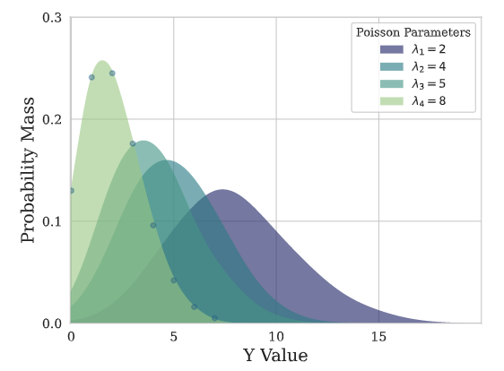
::: {#e4a20e21 .cell 0=‘隐’ 1=‘藏’}
# 单元测试用于检查PMM存储的分位数
# 属性已正确实例化
check = PMM(n_components=2, level=[80, 90])
test_eq(len(check.quantiles), 5)

check = PMM(n_components=2,
            quantiles=[0.0100, 0.1000, 0.5, 0.9000, 0.9900])
print(check.output_names)
print(check.quantiles)
test_eq(len(check.quantiles), 5)

check = PMM(n_components=2,
            quantiles=[0.0100, 0.1000, 0.9000, 0.9900])
test_eq(len(check.quantiles), 4)
:::
# 创建单一混合物并广播至N、H、K
weights = torch.ones((1,3))[None, :, :]
lambdas = torch.Tensor([[5,10,15], [10,20,30]])[None, :, :]

# 为批量维度N创建重复项。
N=2
weights = torch.repeat_interleave(input=weights, repeats=N, dim=0)
lambdas = torch.repeat_interleave(input=lambdas, repeats=N, dim=0)

print('weights.shape (N,H,K) \t', weights.shape)
print('lambdas.shape (N,H,K) \t', lambdas.shape)

distr = PMM(quantiles=[0.1, 0.40, 0.5, 0.60, 0.9])
distr_args = (lambdas,)
samples, sample_mean, quants = distr.sample(distr_args)

print('samples.shape (N,H,num_samples) ', samples.shape)
print('sample_mean.shape (N,H) ', sample_mean.shape)
print('quants.shape  (N,H,Q) \t\t', quants.shape)

# 绘制综合数据
x_plot = range(quants.shape[1]) # H长度
y_plot_hat = quants[0,:,:]  # 过滤器 N,G,T -> H,Q
samples_hat = samples[0,:,:]  # 滤波器 N,G,T -> H,样本数

# 单个预测时间范围 \tau = t+1 的核密度图
fig, ax = plt.subplots(figsize=(3.7, 2.9))

ax.hist(samples_hat[0,:], alpha=0.5, label=r'Horizon $\tau+1$')
ax.hist(samples_hat[1,:], alpha=0.5, label=r'Horizon $\tau+2$')
ax.set(xlabel='Y values', ylabel='Probability')
plt.title('Single horizon Distributions')
plt.legend(bbox_to_anchor=(1, 1), loc='upper left', ncol=1)
plt.grid()
plt.show()
plt.close()

# 绘制模拟轨迹
fig, ax = plt.subplots(figsize=(3.7, 2.9))
plt.plot(x_plot, y_plot_hat[:,2], color='black', label='median [q50]')
plt.fill_between(x_plot,
                 y1=y_plot_hat[:,1], y2=y_plot_hat[:,3],
                 facecolor='blue', alpha=0.4, label='[p25-p75]')
plt.fill_between(x_plot,
                 y1=y_plot_hat[:,0], y2=y_plot_hat[:,4],
                 facecolor='blue', alpha=0.2, label='[p1-p99]')
ax.set(xlabel='Horizon', ylabel='Y values')
plt.title('PMM Probabilistic Predictions')
plt.legend(bbox_to_anchor=(1, 1), loc='upper left', ncol=1)
plt.grid()
plt.show()
plt.close()
高斯混合网格 (GMM)
class GMM(torch.nn.Module):
    """ Gaussian Mixture Mesh

    This Gaussian Mixture statistical model assumes independence across groups of
    data $\mathcal{G}=\{[g_{i}]\}$, and estimates relationships within the group.

    $$ \mathrm{P}\\left(\mathbf{y}_{[b][t+1:t+H]}\\right) =
    \prod_{ [g_{i}] \in \mathcal{G}} \mathrm{P}\left(\mathbf{y}_{[g_{i}][\\tau]}\\right)=
    \prod_{\\beta\in[g_{i}]}
    \\left(\sum_{k=1}^{K} w_k \prod_{(\\beta,\\tau) \in [g_i][t+1:t+H]}
    \mathrm{Gaussian}(y_{\\beta,\\tau}, \hat{\mu}_{\\beta,\\tau,k}, \sigma_{\\beta,\\tau,k})\\right)$$

    **Parameters:**<br>
    `n_components`: int=10, the number of mixture components.<br>
    `level`: float list [0,100], confidence levels for prediction intervals.<br>
    `quantiles`: float list [0,1], alternative to level list, target quantiles.<br>
    `return_params`: bool=False, wether or not return the Distribution parameters.<br>
    `batch_correlation`: bool=False, wether or not model batch correlations.<br>
    `horizon_correlation`: bool=False, wether or not model horizon correlations.<br><br>

    **References:**<br>
    [Kin G. Olivares, O. Nganba Meetei, Ruijun Ma, Rohan Reddy, Mengfei Cao, Lee Dicker.
    Probabilistic Hierarchical Forecasting with Deep Poisson Mixtures. Submitted to the International
    Journal Forecasting, Working paper available at arxiv.](https://arxiv.org/pdf/2110.13179.pdf)
    """
    def __init__(self, n_components=1, level=[80, 90], quantiles=None,
                 num_samples=1000, return_params=False,
                 batch_correlation=False, horizon_correlation=False):
        super(GMM, self).__init__()
        # 将变换级别转换为MQ损失参数
        qs, self.output_names = level_to_outputs(level)
        qs = torch.Tensor(qs)

        # 将分位数转换为同质输出名称
        if quantiles is not None:
            _, self.output_names = quantiles_to_outputs(quantiles)
            qs = torch.Tensor(quantiles)
        self.quantiles = torch.nn.Parameter(qs, requires_grad=False)
        self.num_samples = num_samples
        self.batch_correlation = batch_correlation
        self.horizon_correlation = horizon_correlation

        # If True, predict_step will return Distribution's parameters
        self.return_params = return_params
        if self.return_params:
            mu_names = [f"-mu-{i}" for i in range(1, n_components + 1)]
            std_names = [f"-std-{i}" for i in range(1, n_components + 1)]
            mu_std_names = [i for j in zip(mu_names, std_names) for i in j]
            self.output_names = self.output_names + mu_std_names

        # Add first output entry for the sample_mean
        self.output_names.insert(0, "")

        self.outputsize_multiplier = 2 * n_components
        self.is_distribution_output = True

    def domain_map(self, output: torch.Tensor):
        means, stds = torch.tensor_split(output, 2, dim=-1)
        return (means, stds)

    def scale_decouple(self,
                       output,
                       loc: Optional[torch.Tensor] = None,
                       scale: Optional[torch.Tensor] = None,
                       eps: float=0.2):
        """ Scale Decouple

        Stabilizes model's output optimization, by learning residual
        variance and residual location based on anchoring `loc`, `scale`.
        Also adds domain protection to the distribution parameters.
        """
        means, stds = output
        stds = F.softplus(stds)
        if (loc is not None) and (scale is not None):
            loc = loc.view(means.size(dim=0), 1, -1)
            scale = scale.view(means.size(dim=0), 1, -1)
            means = (means * scale) + loc
            stds = (stds + eps) * scale
        return (means, stds)

    def sample(self, distr_args, num_samples=None):
        """
        Construct the empirical quantiles from the estimated Distribution,
        sampling from it `num_samples` independently.

        **Parameters**<br>
        `distr_args`: Constructor arguments for the underlying Distribution type.<br>
        `loc`: Optional tensor, of the same shape as the batch_shape + event_shape
               of the resulting distribution.<br>
        `scale`: Optional tensor, of the same shape as the batch_shape+event_shape
               of the resulting distribution.<br>
        `num_samples`: int=500, number of samples for the empirical quantiles.<br>

        **Returns**<br>
        `samples`: tensor, shape [B,H,`num_samples`].<br>
        `quantiles`: tensor, empirical quantiles defined by `levels`.<br>
        """
        if num_samples is None:
            num_samples = self.num_samples

        means, stds = distr_args
        B, H, K = means.size()
        Q = len(self.quantiles)
        assert means.shape == stds.shape

        # 样本 K ~ 多项分布(权重)
        # 在B和H之间共享
        # 权重 = torch.repeat_interleave(input=权重, repeats=H, dim=2)

        weights = (1/K) * torch.ones_like(means, device=means.device)

        # 避免循环,向量化
        weights = weights.reshape(-1, K)
        means = means.flatten()
        stds = stds.flatten()

        # 向量化技巧以恢复行索引
        sample_idxs = torch.multinomial(input=weights,
                                        num_samples=num_samples,
                                        replacement=True)
        aux_col_idx = torch.unsqueeze(torch.arange(B * H, device=means.device),-1) * K

        # 去设备
        sample_idxs = sample_idxs.to(means.device)

        sample_idxs = sample_idxs + aux_col_idx
        sample_idxs = sample_idxs.flatten()

        sample_means = means[sample_idxs]
        sample_stds  = stds[sample_idxs]

        # 样本 y ~ 独立地服从正态分布(mu, std)
        samples = torch.normal(sample_means, sample_stds).to(means.device)
        samples = samples.view(B*H, num_samples)
        sample_mean = torch.mean(samples, dim=-1)

        # 计算分位数
        quantiles_device = self.quantiles.to(means.device)
        quants = torch.quantile(input=samples, q=quantiles_device, dim=1)
        quants = quants.permute((1,0)) # Q,B*H

        # 最终重塑
        samples = samples.view(B, H, num_samples)
        sample_mean = sample_mean.view(B, H, 1)
        quants  = quants.view(B, H, Q)

        return samples, sample_mean, quants

    def neglog_likelihood(self,
                          y: torch.Tensor,
                          distr_args: Tuple[torch.Tensor, torch.Tensor],
                          mask: Union[torch.Tensor, None] = None):

        if mask is None:
            mask = torch.ones_like(y)

        means, stds = distr_args
        B, H, K = means.size()

        weights = (1/K) * torch.ones_like(means, device=means.device)

        y = y[:,:, None]
        mask = mask[:,:,None]

        var = stds ** 2
        log_stds = torch.log(stds)
        log_pi = - ((y - means) ** 2 / (2 * var)) - log_stds \
                 - math.log(math.sqrt(2 * math.pi))

        if self.batch_correlation:
            log_pi  = torch.sum(log_pi, dim=0, keepdim=True)

        if self.horizon_correlation:
            log_pi  = torch.sum(log_pi, dim=1, keepdim=True)

        # 数值稳定的混合对数似然
        loglik = torch.logsumexp((torch.log(weights) + log_pi), dim=2, keepdim=True)
        loglik  = loglik * mask

        loss = -torch.mean(loglik)
        return loss

    def __call__(self, y: torch.Tensor,
                 distr_args: Tuple[torch.Tensor, torch.Tensor],
                 mask: Union[torch.Tensor, None] = None,):

        return self.neglog_likelihood(y=y, distr_args=distr_args, mask=mask)
show_doc(GMM, name='GMM.__init__', title_level=3)show_doc(GMM.sample, name='GMM.sample', title_level=3)show_doc(GMM.__call__, name='GMM.__call__', title_level=3)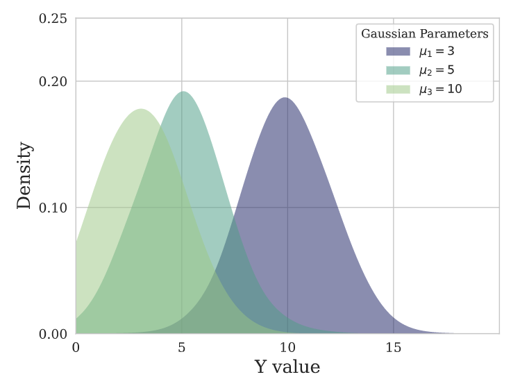
::: {#8ebe4250 .cell 0=‘隐’ 1=‘藏’}
# 单元测试用于检查PMM存储的分位数
# 属性已正确实例化
check = GMM(n_components=2, level=[80, 90])
test_eq(len(check.quantiles), 5)

check = GMM(n_components=2,
            quantiles=[0.0100, 0.1000, 0.5, 0.9000, 0.9900])
print(check.output_names)
print(check.quantiles)
test_eq(len(check.quantiles), 5)

check = GMM(n_components=2,
            quantiles=[0.0100, 0.1000, 0.9000, 0.9900])
test_eq(len(check.quantiles), 4)
:::
# 创建单一混合物并广播至N、H、K
means   = torch.Tensor([[5,10,15], [10,20,30]])[None, :, :]

# 为批处理维度N创建重复项。
N=2
means = torch.repeat_interleave(input=means, repeats=N, dim=0)
weights = torch.ones_like(means)
stds  = torch.ones_like(means)

print('weights.shape (N,H,K) \t', weights.shape)
print('means.shape (N,H,K) \t', means.shape)
print('stds.shape (N,H,K) \t', stds.shape)

distr = GMM(quantiles=[0.1, 0.40, 0.5, 0.60, 0.9])
distr_args = (means, stds)
samples, sample_mean, quants = distr.sample(distr_args)

print('samples.shape (N,H,num_samples) ', samples.shape)
print('sample_mean.shape (N,H) ', sample_mean.shape)
print('quants.shape  (N,H,Q) \t\t', quants.shape)

# 绘制综合数据
x_plot = range(quants.shape[1]) # H长度
y_plot_hat = quants[0,:,:]  # 过滤器 N,G,T -> H,Q
samples_hat = samples[0,:,:]  # 滤波器 N,G,T -> H,num_samples

# 单个预测时间范围 \tau = t+1 的核密度图
fig, ax = plt.subplots(figsize=(3.7, 2.9))

ax.hist(samples_hat[0,:], alpha=0.5, bins=50,
        label=r'Horizon $\tau+1$')
ax.hist(samples_hat[1,:], alpha=0.5, bins=50,
        label=r'Horizon $\tau+2$')
ax.set(xlabel='Y values', ylabel='Probability')
plt.title('Single horizon Distributions')
plt.legend(bbox_to_anchor=(1, 1), loc='upper left', ncol=1)
plt.grid()
plt.show()
plt.close()

# 绘制模拟轨迹
fig, ax = plt.subplots(figsize=(3.7, 2.9))
plt.plot(x_plot, y_plot_hat[:,2], color='black', label='median [q50]')
plt.fill_between(x_plot,
                 y1=y_plot_hat[:,1], y2=y_plot_hat[:,3],
                 facecolor='blue', alpha=0.4, label='[p25-p75]')
plt.fill_between(x_plot,
                 y1=y_plot_hat[:,0], y2=y_plot_hat[:,4],
                 facecolor='blue', alpha=0.2, label='[p1-p99]')
ax.set(xlabel='Horizon', ylabel='Y values')
plt.title('GMM Probabilistic Predictions')
plt.legend(bbox_to_anchor=(1, 1), loc='upper left', ncol=1)
plt.grid()
plt.show()
plt.close()
负二项混合网格 (NBMM)
class NBMM(torch.nn.Module):
    """ Negative Binomial Mixture Mesh

    This N. Binomial Mixture statistical model assumes independence across groups of
    data $\mathcal{G}=\{[g_{i}]\}$, and estimates relationships within the group.

    $$ \mathrm{P}\\left(\mathbf{y}_{[b][t+1:t+H]}\\right) =
    \prod_{ [g_{i}] \in \mathcal{G}} \mathrm{P}\left(\mathbf{y}_{[g_{i}][\\tau]}\\right)=
    \prod_{\\beta\in[g_{i}]}
    \\left(\sum_{k=1}^{K} w_k \prod_{(\\beta,\\tau) \in [g_i][t+1:t+H]}
    \mathrm{NBinomial}(y_{\\beta,\\tau}, \hat{r}_{\\beta,\\tau,k}, \hat{p}_{\\beta,\\tau,k})\\right)$$

    **Parameters:**<br>
    `n_components`: int=10, the number of mixture components.<br>
    `level`: float list [0,100], confidence levels for prediction intervals.<br>
    `quantiles`: float list [0,1], alternative to level list, target quantiles.<br>
    `return_params`: bool=False, wether or not return the Distribution parameters.<br><br>

    **References:**<br>
    [Kin G. Olivares, O. Nganba Meetei, Ruijun Ma, Rohan Reddy, Mengfei Cao, Lee Dicker.
    Probabilistic Hierarchical Forecasting with Deep Poisson Mixtures. Submitted to the International
    Journal Forecasting, Working paper available at arxiv.](https://arxiv.org/pdf/2110.13179.pdf)
    """
    def __init__(self, n_components=1, level=[80, 90], quantiles=None,
                 num_samples=1000, return_params=False):
        super(NBMM, self).__init__()
        # 将变换级别转换为MQLoss参数
        qs, self.output_names = level_to_outputs(level)
        qs = torch.Tensor(qs)

        # 将分位数转换为同质输出名称
        if quantiles is not None:
            _, self.output_names = quantiles_to_outputs(quantiles)
            qs = torch.Tensor(quantiles)
        self.quantiles = torch.nn.Parameter(qs, requires_grad=False)
        self.num_samples = num_samples

        # If True, predict_step will return Distribution's parameters
        self.return_params = return_params
        if self.return_params:
            total_count_names = [f"-total_count-{i}" for i in range(1, n_components + 1)]
            probs_names = [f"-probs-{i}" for i in range(1, n_components + 1)]
            param_names = [i for j in zip(total_count_names, probs_names) for i in j]
            self.output_names = self.output_names + param_names

        # Add first output entry for the sample_mean
        self.output_names.insert(0, "")

        self.outputsize_multiplier = 2 * n_components
        self.is_distribution_output = True

    def domain_map(self, output: torch.Tensor):
        mu, alpha = torch.tensor_split(output, 2, dim=-1)
        return (mu, alpha)

    def scale_decouple(self,
                       output,
                       loc: Optional[torch.Tensor] = None,
                       scale: Optional[torch.Tensor] = None,
                       eps: float=0.2):
        """ Scale Decouple

        Stabilizes model's output optimization, by learning residual
        variance and residual location based on anchoring `loc`, `scale`.
        Also adds domain protection to the distribution parameters.
        """
        # Efficient NBinomial parametrization
        mu, alpha = output
        mu = F.softplus(mu) + 1e-8
        alpha = F.softplus(alpha) + 1e-8    # alpha = 1/total_counts
        if (loc is not None) and (scale is not None):
            loc = loc.view(mu.size(dim=0), 1, -1)
            mu *= loc
            alpha /= (loc + 1.)

        # mu = total_count * (probs/(1-probs))
        # => probs = mu / (total_count + mu)
        # => probs = mu / [total_count * (1 + mu * (1/total_count))]
        total_count = 1.0 / alpha
        probs = (mu * alpha / (1.0 + mu * alpha)) + 1e-8
        return (total_count, probs)

    def sample(self, distr_args, num_samples=None):
        """
        Construct the empirical quantiles from the estimated Distribution,
        sampling from it `num_samples` independently.

        **Parameters**<br>
        `distr_args`: Constructor arguments for the underlying Distribution type.<br>
        `loc`: Optional tensor, of the same shape as the batch_shape + event_shape
               of the resulting distribution.<br>
        `scale`: Optional tensor, of the same shape as the batch_shape+event_shape
               of the resulting distribution.<br>
        `num_samples`: int=500, number of samples for the empirical quantiles.<br>

        **Returns**<br>
        `samples`: tensor, shape [B,H,`num_samples`].<br>
        `quantiles`: tensor, empirical quantiles defined by `levels`.<br>
        """
        if num_samples is None:
            num_samples = self.num_samples

        total_count, probs = distr_args
        B, H, K = total_count.size()
        Q = len(self.quantiles)
        assert total_count.shape == probs.shape

        # 样本 K ~ 多项分布(权重)
        # 在B和H之间共享
        # 权重 = torch.repeat_interleave(input=权重, repeats=H, dim=2)

        weights = (1/K) * torch.ones_like(probs, device=probs.device)

        # 避免循环,向量化
        weights = weights.reshape(-1, K)
        total_count = total_count.flatten()
        probs = probs.flatten()

        # 向量化技巧以恢复行索引
        sample_idxs = torch.multinomial(input=weights,
                                        num_samples=num_samples,
                                        replacement=True)
        aux_col_idx = torch.unsqueeze(torch.arange(B * H, device=probs.device),-1) * K

        # 去设备
        sample_idxs = sample_idxs.to(probs.device)

        sample_idxs = sample_idxs + aux_col_idx
        sample_idxs = sample_idxs.flatten()

        sample_total_count = total_count[sample_idxs]
        sample_probs  = probs[sample_idxs]

        # 样本 y 服从独立负二项分布 NBinomial(total_count, probs)
        dist = NegativeBinomial(total_count=sample_total_count,
                                probs=sample_probs)
        samples = dist.sample(sample_shape=(1,)).to(probs.device)[0]
        samples = samples.view(B*H, num_samples)
        sample_mean = torch.mean(samples, dim=-1)

        # 计算分位数
        quantiles_device = self.quantiles.to(probs.device)
        quants = torch.quantile(input=samples, q=quantiles_device, dim=1)
        quants = quants.permute((1,0)) # Q,B*H

        # 最终重塑
        samples = samples.view(B, H, num_samples)
        sample_mean = sample_mean.view(B, H, 1)
        quants  = quants.view(B, H, Q)

        return samples, sample_mean, quants

    def neglog_likelihood(self,
                          y: torch.Tensor,
                          distr_args: Tuple[torch.Tensor, torch.Tensor],
                          mask: Union[torch.Tensor, None] = None):

        if mask is None:
            mask = torch.ones_like(y)

        total_count, probs = distr_args
        B, H, K = total_count.size()

        weights = (1/K) * torch.ones_like(probs, device=probs.device)

        y = y[:,:, None]
        mask = mask[:,:,None]

        log_unnormalized_prob = (total_count * torch.log(1.-probs) + y * torch.log(probs))
        log_normalization = (-torch.lgamma(total_count + y) + torch.lgamma(1. + y) +
                             torch.lgamma(total_count))
        log_normalization[total_count + y == 0.] = 0.
        log =  log_unnormalized_prob - log_normalization

        # #log = torch.sum(log, dim=0, keepdim=True) 批次/组内联合
        # #log = torch.sum(log, dim=1, keepdim=True) 在预测范围内联合

        # 数值稳定性混合与对数似然
        log_max = torch.amax(log, dim=2, keepdim=True) # [1,1,K](关节塌陷)
        lik     = weights * torch.exp(log-log_max)     # 取最大值
        loglik  = torch.log(torch.sum(lik, dim=2, keepdim=True)) + log_max # 返回最大值

        loglik  = loglik * mask #替换为掩码

        loss = -torch.mean(loglik)
        return loss

    def __call__(self, y: torch.Tensor,
                 distr_args: Tuple[torch.Tensor, torch.Tensor],
                 mask: Union[torch.Tensor, None] = None,):

        return self.neglog_likelihood(y=y, distr_args=distr_args, mask=mask)
show_doc(NBMM, name='NBMM.__init__', title_level=3)show_doc(NBMM.sample, name='NBMM.sample', title_level=3)show_doc(NBMM.__call__, name='NBMM.__call__', title_level=3)# 创建单一混合物并广播至N、H、K
counts = torch.Tensor([[10,20,30], [20,40,60]])[None, :, :]
# 为批处理维度N创建重复项。
N=2
counts = torch.repeat_interleave(input=counts, repeats=N, dim=0)
weights = torch.ones_like(counts)
probs = torch.ones_like(counts) * 0.5
print('weights.shape (N,H,K) \t', weights.shape)
print('counts.shape (N,H,K) \t', counts.shape)
print('probs.shape (N,H,K) \t', probs.shape)
model = NBMM(quantiles=[0.1, 0.40, 0.5, 0.60, 0.9])
distr_args = (counts, probs)
samples, sample_mean, quants = model.sample(distr_args, num_samples=2000)
print('samples.shape (N,H,num_samples) ', samples.shape)
print('sample_mean.shape (N,H) ', sample_mean.shape)
print('quants.shape (N,H,Q) \t\t', quants.shape)
# 绘制综合数据
x_plot = range(quants.shape[1]) # H长度
y_plot_hat = quants[0,:,:] # 过滤器 N,G,T -> H,Q
samples_hat = samples[0,:,:] # 滤波器 N,G,T -> H,num_samples
# 单个预测时间范围 \tau = t+1 的核密度图
fig, ax = plt.subplots(figsize=(3.7, 2.9))
ax.hist(samples_hat[0,:], alpha=0.5, bins=30,
label=r'Horizon $\tau+1$')
ax.hist(samples_hat[1,:], alpha=0.5, bins=30,
label=r'Horizon $\tau+2$')
ax.set(xlabel='Y values', ylabel='Probability')
plt.title('Single horizon Distributions')
plt.legend(bbox_to_anchor=(1, 1), loc='upper left', ncol=1)
plt.grid()
plt.show()
plt.close()
# 绘制模拟轨迹
fig, ax = plt.subplots(figsize=(3.7, 2.9))
plt.plot(x_plot, y_plot_hat[:,2], color='black', label='median [q50]')
plt.fill_between(x_plot,
y1=y_plot_hat[:,1], y2=y_plot_hat[:,3],
facecolor='blue', alpha=0.4, label='[p25-p75]')
plt.fill_between(x_plot,
y1=y_plot_hat[:,0], y2=y_plot_hat[:,4],
facecolor='blue', alpha=0.2, label='[p1-p99]')
ax.set(xlabel='Horizon', ylabel='Y values')
plt.title('NBM Probabilistic Predictions')
plt.legend(bbox_to_anchor=(1, 1), loc='upper left', ncol=1)
plt.grid()
plt.show()
plt.close()5. 强健化错误
这种来自强健统计的错误类型关注于对异常值和假设违反具有抵抗力的方法,提供可靠的估计和推断。强健估计量用于减少异常值的影响,提供更稳定的结果。
Huber 损失
class HuberLoss(BasePointLoss):
    """ Huber Loss

    The Huber loss, employed in robust regression, is a loss function that
    exhibits reduced sensitivity to outliers in data when compared to the
    squared error loss. This function is also refered as SmoothL1.

    The Huber loss function is quadratic for small errors and linear for large
    errors, with equal values and slopes of the different sections at the two
    points where $(y_{\\tau}-\hat{y}_{\\tau})^{2}$=$|y_{\\tau}-\hat{y}_{\\tau}|$.

    $$ L_{\delta}(y_{\\tau},\; \hat{y}_{\\tau})
    =\\begin{cases}{\\frac{1}{2}}(y_{\\tau}-\hat{y}_{\\tau})^{2}\;{\\text{for }}|y_{\\tau}-\hat{y}_{\\tau}|\leq \delta \\\
    \\delta \ \cdot \left(|y_{\\tau}-\hat{y}_{\\tau}|-{\\frac {1}{2}}\delta \\right),\;{\\text{otherwise.}}\end{cases}$$

    where $\\delta$ is a threshold parameter that determines the point at which the loss transitions from quadratic to linear,
    and can be tuned to control the trade-off between robustness and accuracy in the predictions.

    **Parameters:**<br>
    `delta`: float=1.0, Specifies the threshold at which to change between delta-scaled L1 and L2 loss.
    `horizon_weight`: Tensor of size h, weight for each timestamp of the forecasting window. <br>

    **References:**<br>
    [Huber Peter, J (1964). "Robust Estimation of a Location Parameter". Annals of Statistics](https://projecteuclid.org/journals/annals-of-mathematical-statistics/volume-35/issue-1/Robust-Estimation-of-a-Location-Parameter/10.1214/aoms/1177703732.full)
    """
    def __init__(self, delta: float=1., horizon_weight=None):
        super(HuberLoss, self).__init__(horizon_weight=horizon_weight,
                                  outputsize_multiplier=1,
                                  output_names=[''])
        self.delta = delta

    def __call__(self,
                 y: torch.Tensor,
                 y_hat: torch.Tensor,
                 mask: Union[torch.Tensor, None] = None):
        """
        **Parameters:**<br>
        `y`: tensor, Actual values.<br>
        `y_hat`: tensor, Predicted values.<br>
        `mask`: tensor, Specifies date stamps per serie to consider in loss.<br>

        **Returns:**<br>
        `huber_loss`: tensor (single value).
        """
        losses = F.huber_loss(y, y_hat, reduction='none', delta=self.delta)
        weights = self._compute_weights(y=y, mask=mask)
        return _weighted_mean(losses=losses, weights=weights)
show_doc(HuberLoss, name='HuberLoss.__init__', title_level=3)show_doc(HuberLoss.__call__, name='HuberLoss.__call__', title_level=3)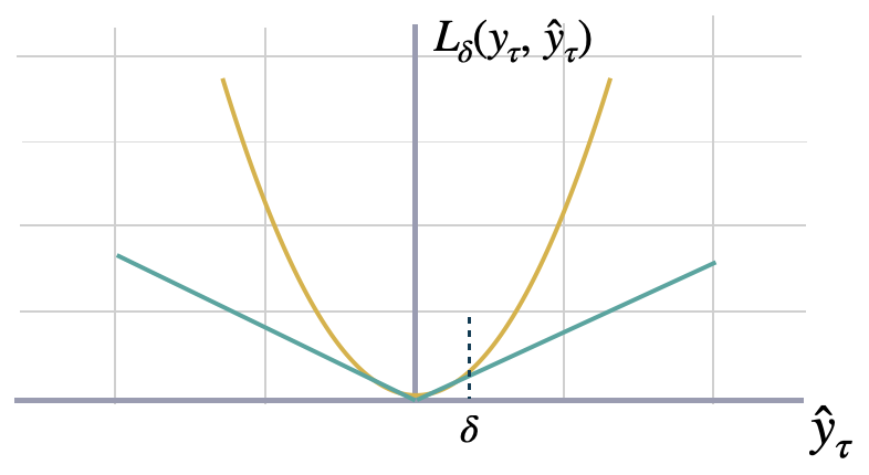
图基损失
class TukeyLoss(torch.nn.Module):
    """ Tukey Loss

    The Tukey loss function, also known as Tukey's biweight function, is a
    robust statistical loss function used in robust statistics. Tukey's loss exhibits
    quadratic behavior near the origin, like the Huber loss; however, it is even more
    robust to outliers as the loss for large residuals remains constant instead of
    scaling linearly.

    The parameter $c$ in Tukey's loss determines the ''saturation'' point
    of the function: Higher values of $c$ enhance sensitivity, while lower values
    increase resistance to outliers.

    $$ L_{c}(y_{\\tau},\; \hat{y}_{\\tau})
    =\\begin{cases}{
    \\frac{c^{2}}{6}} \\left[1-(\\frac{y_{\\tau}-\hat{y}_{\\tau}}{c})^{2} \\right]^{3}    \;\\text{for } |y_{\\tau}-\hat{y}_{\\tau}|\leq c \\\
    \\frac{c^{2}}{6} \qquad \\text{otherwise.}  \end{cases}$$

    Please note that the Tukey loss function assumes the data to be stationary or
    normalized beforehand. If the error values are excessively large, the algorithm
    may need help to converge during optimization. It is advisable to employ small learning rates.

    **Parameters:**<br>
    `c`: float=4.685, Specifies the Tukey loss' threshold on which residuals are no longer considered.<br>
    `normalize`: bool=True, Wether normalization is performed within Tukey loss' computation.<br>

    **References:**<br>
    [Beaton, A. E., and Tukey, J. W. (1974). "The Fitting of Power Series, Meaning Polynomials, Illustrated on Band-Spectroscopic Data."](https://www.jstor.org/stable/1267936)
    """
    def __init__(self, c: float=4.685, normalize: bool=True):
        super(TukeyLoss, self).__init__()
        self.outputsize_multiplier = 1
        self.c = c
        self.normalize = normalize
        self.output_names = ['']
        self.is_distribution_output = False

    def domain_map(self, y_hat: torch.Tensor):
        """
        单变量损失在维度 [B,T,H] 或 [B,H] 上进行操作
        这使得网络的输出从 [B,H,1] 变为 [B,H]
        """
        return y_hat.squeeze(-1)

    def masked_mean(self, x, mask, dim):
        x_nan = x.masked_fill(mask < 1, float("nan"))
        x_mean = x_nan.nanmean(dim=dim, keepdim=True)
        x_mean = torch.nan_to_num(x_mean, nan=0.0)
        return x_mean

    def __call__(self, y: torch.Tensor, y_hat: torch.Tensor,
                 mask: Union[torch.Tensor, None] = None):
        """
        **Parameters:**<br>
        `y`: tensor, Actual values.<br>
        `y_hat`: tensor, Predicted values.<br>
        `mask`: tensor, Specifies date stamps per serie to consider in loss.<br>

        **Returns:**<br>
        `tukey_loss`: tensor (single value).
        """
        if mask is None:
            mask = torch.ones_like(y_hat)

        # 我们对Tukey损失进行了归一化处理,以满足4.685的正态异常值界限。
        if self.normalize:
            y_mean = self.masked_mean(x=y, mask=mask, dim=-1)
            y_std = torch.sqrt(self.masked_mean(x=(y - y_mean) ** 2, mask=mask, dim=-1)) + 1e-2
        else:
            y_std = 1.
        delta_y = torch.abs(y - y_hat) / y_std

        tukey_mask = torch.greater_equal(self.c * torch.ones_like(delta_y), delta_y)
        tukey_loss = tukey_mask * mask * (1-(delta_y/(self.c))**2)**3 + (1-(tukey_mask * 1))
        tukey_loss = (self.c**2 / 6) * torch.mean(tukey_loss)
        return tukey_loss
show_doc(TukeyLoss, name='TukeyLoss.__init__', title_level=3)show_doc(TukeyLoss.__call__, name='TukeyLoss.__call__', title_level=3)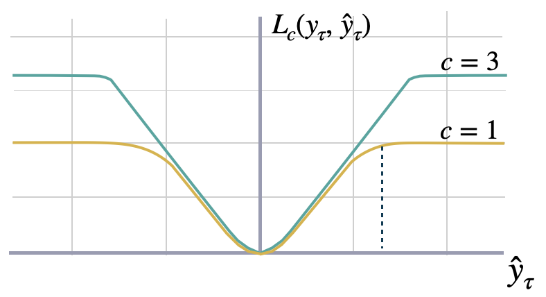
Huber化的分位数损失
class HuberQLoss(BasePointLoss):
    """ Huberized Quantile Loss

    The Huberized quantile loss is a modified version of the quantile loss function that
    combines the advantages of the quantile loss and the Huber loss. It is commonly used
    in regression tasks, especially when dealing with data that contains outliers or heavy tails.

    The Huberized quantile loss between `y` and `y_hat` measure the Huber Loss in a non-symmetric way.
    The loss pays more attention to under/over-estimation depending on the quantile parameter $q$;
    and controls the trade-off between robustness and accuracy in the predictions with the parameter $delta$.

    $$ \mathrm{HuberQL}(\\mathbf{y}_{\\tau}, \\mathbf{\hat{y}}^{(q)}_{\\tau}) =
    (1-q)\, L_{\delta}(y_{\\tau},\; \hat{y}^{(q)}_{\\tau}) \mathbb{1}\{ \hat{y}^{(q)}_{\\tau} \geq y_{\\tau} \} +
    q\, L_{\delta}(y_{\\tau},\; \hat{y}^{(q)}_{\\tau}) \mathbb{1}\{ \hat{y}^{(q)}_{\\tau} < y_{\\tau} \} $$

    **Parameters:**<br>
    `delta`: float=1.0, Specifies the threshold at which to change between delta-scaled L1 and L2 loss.<br>
    `q`: float, between 0 and 1. The slope of the quantile loss, in the context of quantile regression, the q determines the conditional quantile level.<br>
    `horizon_weight`: Tensor of size h, weight for each timestamp of the forecasting window. <br>

    **References:**<br>
    [Huber Peter, J (1964). "Robust Estimation of a Location Parameter". Annals of Statistics](https://projecteuclid.org/journals/annals-of-mathematical-statistics/volume-35/issue-1/Robust-Estimation-of-a-Location-Parameter/10.1214/aoms/1177703732.full)<br>
    [Roger Koenker and Gilbert Bassett, Jr., "Regression Quantiles".](https://www.jstor.org/stable/1913643)
    """
    def __init__(self, q, delta: float=1., horizon_weight=None):
        super(HuberQLoss, self).__init__(horizon_weight=horizon_weight,
                                           outputsize_multiplier=1,
                                           output_names=[f'_q{q}_d{delta}'])
        self.q = q
        self.delta = delta

    def __call__(self,
                 y: torch.Tensor,
                 y_hat: torch.Tensor,
                 mask: Union[torch.Tensor, None] = None):
        """
        **Parameters:**<br>
        `y`: tensor, Actual values.<br>
        `y_hat`: tensor, Predicted values.<br>
        `mask`: tensor, Specifies datapoints to consider in loss.<br>

        **Returns:**<br>
        `huber_qloss`: tensor (single value).
        """
        error  = y_hat - y
        zero_error = torch.zeros_like(error)
        sq     = torch.maximum(-error, zero_error)
        s1_q   = torch.maximum(error, zero_error)
        losses = self.q * F.huber_loss(sq, zero_error,
                                       reduction='none', delta=self.delta) + \
                 (1 - self.q) * F.huber_loss(s1_q, zero_error,
                                        reduction='none', delta=self.delta)

        weights = self._compute_weights(y=y, mask=mask)
        return _weighted_mean(losses=losses, weights=weights)
show_doc(HuberQLoss, name='HuberQLoss.__init__', title_level=3)show_doc(HuberQLoss.__call__, name='HuberQLoss.__call__', title_level=3)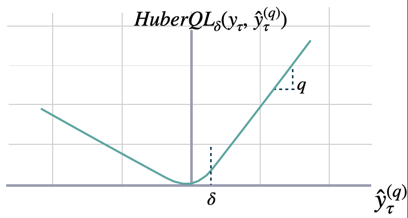
Huber化的MQLoss
class HuberMQLoss(BasePointLoss):
    """  Huberized Multi-Quantile loss

    The Huberized Multi-Quantile loss (HuberMQL) is a modified version of the multi-quantile loss function
    that combines the advantages of the quantile loss and the Huber loss. HuberMQL is commonly used in regression
    tasks, especially when dealing with data that contains outliers or heavy tails. The loss function pays
    more attention to under/over-estimation depending on the quantile list $[q_{1},q_{2},\dots]$ parameter.
    It controls the trade-off between robustness and prediction accuracy with the parameter $\\delta$.

    $$ \mathrm{HuberMQL}_{\delta}(\\mathbf{y}_{\\tau},[\\mathbf{\hat{y}}^{(q_{1})}_{\\tau}, ... ,\hat{y}^{(q_{n})}_{\\tau}]) =
    \\frac{1}{n} \\sum_{q_{i}} \mathrm{HuberQL}_{\\delta}(\\mathbf{y}_{\\tau}, \\mathbf{\hat{y}}^{(q_{i})}_{\\tau}) $$

    **Parameters:**<br>
    `level`: int list [0,100]. Probability levels for prediction intervals (Defaults median).
    `quantiles`: float list [0., 1.]. Alternative to level, quantiles to estimate from y distribution.
    `delta`: float=1.0, Specifies the threshold at which to change between delta-scaled L1 and L2 loss.<br>
    `horizon_weight`: Tensor of size h, weight for each timestamp of the forecasting window. <br>

    **References:**<br>
    [Huber Peter, J (1964). "Robust Estimation of a Location Parameter". Annals of Statistics](https://projecteuclid.org/journals/annals-of-mathematical-statistics/volume-35/issue-1/Robust-Estimation-of-a-Location-Parameter/10.1214/aoms/1177703732.full)<br>
    [Roger Koenker and Gilbert Bassett, Jr., "Regression Quantiles".](https://www.jstor.org/stable/1913643)
    """
    def __init__(self, level=[80, 90], quantiles=None, delta: float=1.0, horizon_weight=None):

        qs, output_names = level_to_outputs(level)
        qs = torch.Tensor(qs)
        # 将分位数转换为同质输出名称
        if quantiles is not None:
            _, output_names = quantiles_to_outputs(quantiles)
            qs = torch.Tensor(quantiles)

        super(HuberMQLoss, self).__init__(horizon_weight=horizon_weight,
                                     outputsize_multiplier=len(qs),
                                     output_names=output_names)

        self.quantiles = torch.nn.Parameter(qs, requires_grad=False)
        self.delta = delta

    def domain_map(self, y_hat: torch.Tensor):
        """
        身份域映射 [B,T,H,Q]/[B,H,Q]
        """
        return y_hat

    def _compute_weights(self, y, mask):
        """
        Compute final weights for each datapoint (based on all weights and all masks)
        Set horizon_weight to a ones[H] tensor if not set.
        If set, check that it has the same length as the horizon in x.
        """
        if mask is None:
            mask = torch.ones_like(y, device=y.device)
        else:
            mask = mask.unsqueeze(1) # 添加Q维度。

        if self.horizon_weight is None:
            self.horizon_weight = torch.ones(mask.shape[-1])
        else:
            assert mask.shape[-1] == len(self.horizon_weight), \
                'horizon_weight must have same length as Y'

        weights = self.horizon_weight.clone()
        weights = torch.ones_like(mask, device=mask.device) * weights.to(mask.device)
        return weights * mask

    def __call__(self,
                 y: torch.Tensor,
                 y_hat: torch.Tensor,
                 mask: Union[torch.Tensor, None] = None):
        """
        **Parameters:**<br>
        `y`: tensor, Actual values.<br>
        `y_hat`: tensor, Predicted values.<br>
        `mask`: tensor, Specifies date stamps per serie to consider in loss.<br>

        **Returns:**<br>
        `hmqloss`: tensor (single value).
        """

        error  = y_hat - y.unsqueeze(-1)
        zero_error = torch.zeros_like(error)
        sq     = torch.maximum(-error, torch.zeros_like(error))
        s1_q   = torch.maximum(error, torch.zeros_like(error))
        losses = F.huber_loss(self.quantiles * sq, zero_error,
                                        reduction='none', delta=self.delta) + \
                  F.huber_loss((1 - self.quantiles) * s1_q, zero_error,
                                reduction='none', delta=self.delta)
        losses = (1/len(self.quantiles)) * losses

        if y_hat.ndim == 3: # 基础窗口
            losses = losses.swapaxes(-2,-1) # [B,H,Q] -> [B,Q,H](用于水平加权,H置于末尾)
        elif y_hat.ndim == 4: # 基础循环
            losses = losses.swapaxes(-2,-1)
            losses = losses.swapaxes(-2,-3) # [B,seq_len,H,Q] -> [B,Q,seq_len,H] (用于水平加权,H置于末尾)

        weights = self._compute_weights(y=losses, mask=mask) # 利用损失增加暗度
        # 注意:权重没有Q维度。

        return _weighted_mean(losses=losses, weights=weights)
show_doc(HuberMQLoss, name='HuberMQLoss.__init__', title_level=3)show_doc(HuberMQLoss.__call__, name='HuberMQLoss.__call__', title_level=3)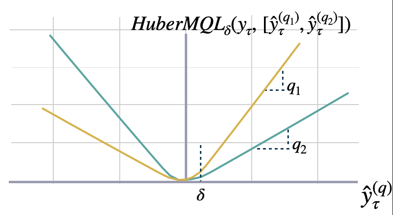
6. 其他
准确性
class Accuracy(torch.nn.Module):
    """ Accuracy

    Computes the accuracy between categorical `y` and `y_hat`.
    This evaluation metric is only meant for evalution, as it
    is not differentiable.

    $$ \mathrm{Accuracy}(\\mathbf{y}_{\\tau}, \\mathbf{\hat{y}}_{\\tau}) = \\frac{1}{H} \\sum^{t+H}_{\\tau=t+1} \mathrm{1}\{\\mathbf{y}_{\\tau}==\\mathbf{\hat{y}}_{\\tau}\} $$

    """
    def __init__(self,):
        super(Accuracy, self).__init__()
        self.is_distribution_output = False

    def domain_map(self, y_hat: torch.Tensor):
        """
        单变量损失在维度 [B,T,H]/[B,H] 上进行操作
        这使得网络的输出从 [B,H,1] 变为 [B,H]
        """
        return y_hat.squeeze(-1)

    def __call__(self, y: torch.Tensor, y_hat: torch.Tensor,
                 mask: Union[torch.Tensor, None] = None):
        """
        **Parameters:**<br>
        `y`: tensor, Actual values.<br>
        `y_hat`: tensor, Predicted values.<br>
        `mask`: tensor, Specifies date stamps per serie to consider in loss.<br>

        **Returns:**<br>
        `accuracy`: tensor (single value).
        """
        if mask is None:
            mask = torch.ones_like(y_hat)

        measure = (y.unsqueeze(-1) == y_hat) * mask.unsqueeze(-1)
        accuracy = torch.mean(measure)
        return accuracy
show_doc(Accuracy, name='Accuracy.__init__', title_level=3)show_doc(Accuracy.__call__, name='Accuracy.__call__', title_level=3)缩放的连续排名概率评分 (sCRPS)
class sCRPS(torch.nn.Module):
    """Scaled Continues Ranked Probability Score

    Calculates a scaled variation of the CRPS, as proposed by Rangapuram (2021),
    to measure the accuracy of predicted quantiles `y_hat` compared to the observation `y`.

    This metric averages percentual weighted absolute deviations as
    defined by the quantile losses.

    $$ \mathrm{sCRPS}(\\mathbf{\hat{y}}^{(q)}_{\\tau}, \mathbf{y}_{\\tau}) = \\frac{2}{N} \sum_{i}
    \int^{1}_{0}
    \\frac{\mathrm{QL}(\\mathbf{\hat{y}}^{(q}_{\\tau} y_{i,\\tau})_{q}}{\sum_{i} | y_{i,\\tau} |} dq $$

    where $\\mathbf{\hat{y}}^{(q}_{\\tau}$ is the estimated quantile, and $y_{i,\\tau}$
    are the target variable realizations.

    **Parameters:**<br>
    `level`: int list [0,100]. Probability levels for prediction intervals (Defaults median).
    `quantiles`: float list [0., 1.]. Alternative to level, quantiles to estimate from y distribution.

    **References:**<br>
    - [Gneiting, Tilmann. (2011). \"Quantiles as optimal point forecasts\".
    International Journal of Forecasting.](https://www.sciencedirect.com/science/article/pii/S0169207010000063)<br>
    - [Spyros Makridakis, Evangelos Spiliotis, Vassilios Assimakopoulos, Zhi Chen, Anil Gaba, Ilia Tsetlin, Robert L. Winkler. (2022).
    \"The M5 uncertainty competition: Results, findings and conclusions\".
    International Journal of Forecasting.](https://www.sciencedirect.com/science/article/pii/S0169207021001722)<br>
    - [Syama Sundar Rangapuram, Lucien D Werner, Konstantinos Benidis, Pedro Mercado, Jan Gasthaus, Tim Januschowski. (2021).
    \"End-to-End Learning of Coherent Probabilistic Forecasts for Hierarchical Time Series\".
    Proceedings of the 38th International Conference on Machine Learning (ICML).](https://proceedings.mlr.press/v139/rangapuram21a.html)
    """
    def __init__(self, level=[80, 90], quantiles=None):
        super(sCRPS, self).__init__()
        self.mql = MQLoss(level=level, quantiles=quantiles)
        self.is_distribution_output = False

    def __call__(self, y: torch.Tensor, y_hat: torch.Tensor,
                 mask: Union[torch.Tensor, None] = None):
        """
        **Parameters:**<br>
        `y`: tensor, Actual values.<br>
        `y_hat`: tensor, Predicted values.<br>
        `mask`: tensor, Specifies date stamps per series to consider in loss.<br>

        **Returns:**<br>
        `scrps`: tensor (single value).
        """
        mql = self.mql(y=y, y_hat=y_hat, mask=mask)
        norm = torch.sum(torch.abs(y))
        unmean = torch.sum(mask)
        scrps = 2 * mql * unmean / (norm + 1e-5)
        return scrps
show_doc(sCRPS, name='sCRPS.__init__', title_level=3)show_doc(sCRPS.__call__, name='sCRPS.__call__', title_level=3)# 每个1代表一个错误,共有6个数据点。
y = torch.Tensor([[0,0,0],[0,0,0]])
y_hat = torch.Tensor([[0,0,1],[1,0,1]])
# 完整掩码和地平线权重
mask = torch.Tensor([[1,1,1],[1,1,1]])
horizon_weight = torch.Tensor([1,1,1])
mae = MAE(horizon_weight=horizon_weight)
loss = mae(y=y, y_hat=y_hat, mask=mask)
assert loss==(3/6), 'Should be 3/6'
# 不完整掩码与完整地平线权重
mask = torch.Tensor([[1,1,1],[0,1,1]]) # 仅1个错误和点被屏蔽。
horizon_weight = torch.Tensor([1,1,1])
mae = MAE(horizon_weight=horizon_weight)
loss = mae(y=y, y_hat=y_hat, mask=mask)
assert loss==(2/5), 'Should be 2/5'
# 完整面具与不完全地平线_权重
mask = torch.Tensor([[1,1,1],[1,1,1]])
horizon_weight = torch.Tensor([1,1,0]) # 2个错误和点被屏蔽。
mae = MAE(horizon_weight=horizon_weight)
loss = mae(y=y, y_hat=y_hat, mask=mask)
assert loss==(1/4), 'Should be 1/4'
# 不完整的掩码和不完整的地平线权重
mask = torch.Tensor([[0,1,1],[1,1,1]])
horizon_weight = torch.Tensor([1,1,0]) # 2个错误被掩盖,扣3分。
mae = MAE(horizon_weight=horizon_weight)
loss = mae(y=y, y_hat=y_hat, mask=mask)
assert loss==(1/3), 'Should be 1/3'Give us a ⭐ on Github