from typing import Tuple, Optional

import torch
import torch.nn as nn
import torch.nn.functional as F
from torch import Tensor
from torch.nn import LayerNorm
import pandas as pd
from neuralforecast.losses.pytorch import MAE
from neuralforecast.common._base_windows import BaseWindowsTFT
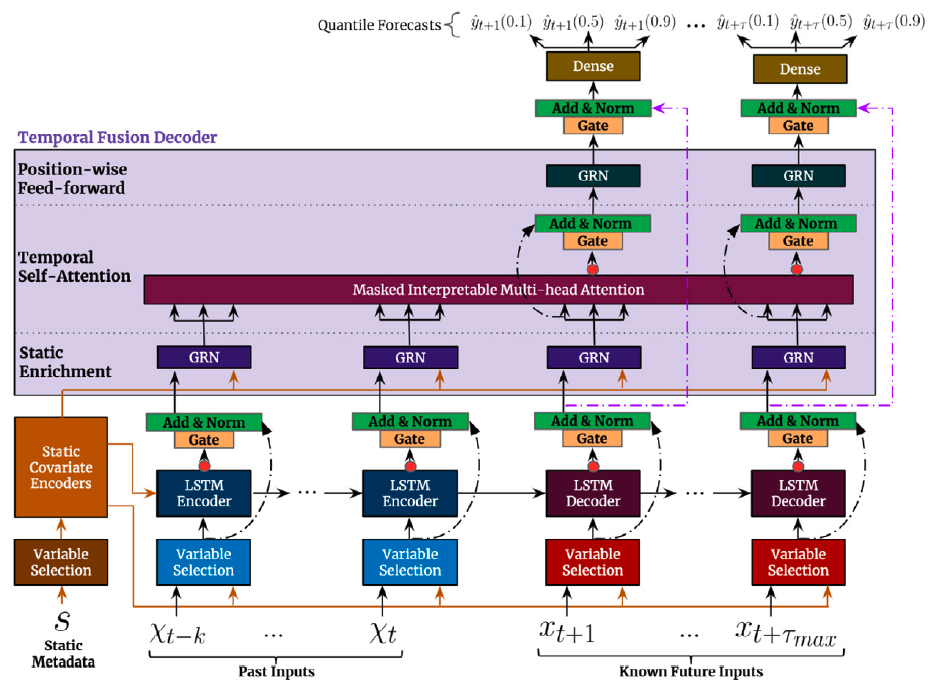
总之,时间融合变换器(TFT)结合了门控层、LSTM递归编码器和多头注意力层,形成了一种多步预测策略解码器。
TFT的输入包括静态外生变量 \(\mathbf{x}^{(s)}\)、历史外生变量 \(\mathbf{x}^{(h)}_{[:t]}\)、预测时可用的外生变量 \(\mathbf{x}^{(f)}_{[:t+H]}\) 和自回归特征 \(\mathbf{y}_{[:t]}\),这些输入进一步分解为分类和连续特征。该网络使用多量纲回归来建模以下条件概率:\[\mathbb{P}(\mathbf{y}_{[t+1:t+H]}|\;\mathbf{y}_{[:t]},\; \mathbf{x}^{(h)}_{[:t]},\; \mathbf{x}^{(f)}_{[:t+H]},\; \mathbf{x}^{(s)})\]
参考文献
- Jan Golda, Krzysztof Kudrynski. “NVIDIA, 深度学习预测示例”
- Bryan Lim, Sercan O. Arik, Nicolas Loeff, Tomas Pfister, “时间融合变换器用于可解释的多视野时间序列预测”
import logging
import warnings

from fastcore.test import test_eq
from nbdev.showdoc import show_doclogging.getLogger("pytorch_lightning").setLevel(logging.ERROR)
warnings.filterwarnings("ignore")1. 辅助函数
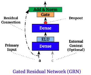
1.1 门控机制
门控残差网络(GRN)提供了自适应的深度和网络复杂性,能够适应不同大小的数据集。由于残差连接允许网络跳过输入 \(\mathbf{a}\) 和上下文 \(\mathbf{c}\) 的非线性变换。
\[\begin{align} \eta_{1} &= \mathrm{ELU}(\mathbf{W}_{1}\mathbf{a}+\mathbf{W}_{2}\mathbf{c}+\mathbf{b}_{1}) \\ \eta_{2} &= \mathbf{W}_{2}\eta_{1}+b_{2} \\ \mathrm{GRN}(\mathbf{a}, \mathbf{c}) &= \mathrm{LayerNorm}(a + \textrm{GLU}(\eta_{2})) \end{align}\]
门控线性单元(GLU)提供了抑制 GRN 中不必要部分的灵活性。考虑 GRN 的输出 \(\gamma\),那么 GLU 变换定义为:
\[\mathrm{GLU}(\gamma) = \sigma(\mathbf{W}_{4}\gamma +b_{4}) \odot (\mathbf{W}_{5}\gamma +b_{5})\]
class MaybeLayerNorm(nn.Module):
    def __init__(self, output_size, hidden_size, eps):
        super().__init__()
        if output_size and output_size == 1:
            self.ln = nn.Identity()
        else:
            self.ln = LayerNorm(output_size if output_size else hidden_size,
                                eps=eps)

    def forward(self, x):
        return self.ln(x)

class GLU(nn.Module):
    def __init__(self, hidden_size, output_size):
        super().__init__()
        self.lin = nn.Linear(hidden_size, output_size * 2)

    def forward(self, x: Tensor) -> Tensor:
        x = self.lin(x)
        x = F.glu(x)
        return x

class GRN(nn.Module):
    def __init__(self,
                 input_size,
                 hidden_size,
                 output_size=None,
                 context_hidden_size=None,
                 dropout=0):
        super().__init__()

        self.layer_norm = MaybeLayerNorm(output_size, hidden_size, eps=1e-3)
        self.lin_a = nn.Linear(input_size, hidden_size)
        if context_hidden_size is not None:
            self.lin_c = nn.Linear(context_hidden_size, hidden_size, bias=False)
        self.lin_i = nn.Linear(hidden_size, hidden_size)
        self.glu = GLU(hidden_size, output_size if output_size else hidden_size)
        self.dropout = nn.Dropout(dropout)
        self.out_proj = nn.Linear(input_size, output_size) if output_size else None

    def forward(self, a: Tensor, c: Optional[Tensor] = None):
        x = self.lin_a(a)
        if c is not None:
            x = x + self.lin_c(c).unsqueeze(1)
        x = F.elu(x)
        x = self.lin_i(x)
        x = self.dropout(x)
        x = self.glu(x)
        y = a if not self.out_proj else self.out_proj(a)
        x = x + y
        x = self.layer_norm(x)
        return x
1.2 变量选择网络
TFT 通过其变量选择网络 (VSN) 组件包含自动变量选择能力。VSN 接收原始输入 \(\{\mathbf{x}^{(s)}, \mathbf{x}^{(h)}_{[:t]}, \mathbf{x}^{(f)}_{[:t]}\}\),并通过嵌入或线性变换将其转换到高维空间 \(\{\mathbf{E}^{(s)}, \mathbf{E}^{(h)}_{[:t]}, \mathbf{E}^{(f)}_{[:t+H]}\}\)。
对于观察到的历史数据,时间 \(t\) 时的嵌入矩阵 \(\mathbf{E}^{(h)}_{t}\) 是 \(j\) 个变量 \(e^{(h)}_{t,j}\) 嵌入的连接: \[\begin{align} \mathbf{E}^{(h)}_{t} &= [e^{(h)}_{t,1},\dots,e^{(h)}_{t,j},\dots,e^{(h)}_{t,n_{h}}] \\ \mathbf{\tilde{e}}^{(h)}_{t,j} &= \mathrm{GRN}(e^{(h)}_{t,j}) \end{align}\]
变量选择权重由以下公式给出: \[s^{(h)}_{t}=\mathrm{SoftMax}(\mathrm{GRN}(\mathbf{E}^{(h)}_{t},\mathbf{E}^{(s)}))\]
然后处理后的 VSN 特征为: \[\tilde{\mathbf{E}}^{(h)}_{t}= \sum_{j} s^{(h)}_{j} \tilde{e}^{(h)}_{t,j}\]

class TFTEmbedding(nn.Module):
    def __init__(self, hidden_size, stat_input_size, futr_input_size, hist_input_size, tgt_size):
        super().__init__()
        # 输入类型有四种:
        # 1. 静态连续
        # 2. 先验已知的时间连续性
        # 3. 时间观察连续性
        # 4. 时间观察目标(迄今为止的时间序列观察结果)

        self.hidden_size = hidden_size

        self.stat_input_size = stat_input_size
        self.futr_input_size = futr_input_size
        self.hist_input_size = hist_input_size
        self.tgt_size        = tgt_size

        # 如果大小不为None,则实例化连续嵌入。
        for attr, size in [('stat_exog_embedding', stat_input_size),
                           ('futr_exog_embedding', futr_input_size),
                           ('hist_exog_embedding', hist_input_size),
                           ('tgt_embedding', tgt_size)]:
            if size:
                vectors = nn.Parameter(torch.Tensor(size, hidden_size))
                bias = nn.Parameter(torch.zeros(size, hidden_size))
                torch.nn.init.xavier_normal_(vectors)
                setattr(self, attr+'_vectors', vectors)
                setattr(self, attr+'_bias', bias)
            else:
                setattr(self, attr+'_vectors', None)
                setattr(self, attr+'_bias', None)

    def _apply_embedding(self,
                         cont: Optional[Tensor],
                         cont_emb: Tensor,
                         cont_bias: Tensor,
                         ):

        if (cont is not None):
            #下面的代码等价于以下einsums
            #e_cont = torch.einsum('btf,fh->bthf', cont, cont_emb)
            #e_cont = torch.einsum('bf,fh->bhf', cont, cont_emb)
            e_cont = torch.mul(cont.unsqueeze(-1), cont_emb)
            e_cont = e_cont + cont_bias
            return e_cont

        return None

    def forward(self, target_inp,
                stat_exog=None, futr_exog=None, hist_exog=None):
        # 时间/静态 分类/连续 已知/观察到的 输入
        # 尝试获取输入,如果失败则返回None。

        # 静态输入在所有时间步长中应保持一致。
        # 为了提高内存效率,没有使用断言语句。
        stat_exog = stat_exog[:,:] if stat_exog is not None else None

        s_inp = self._apply_embedding(cont=stat_exog,
                                      cont_emb=self.stat_exog_embedding_vectors,
                                      cont_bias=self.stat_exog_embedding_bias)
        k_inp = self._apply_embedding(cont=futr_exog,
                                      cont_emb=self.futr_exog_embedding_vectors,
                                      cont_bias=self.futr_exog_embedding_bias)
        o_inp = self._apply_embedding(cont=hist_exog,
                                      cont_emb=self.hist_exog_embedding_vectors,
                                      cont_bias=self.hist_exog_embedding_bias)

        # 时间观测目标
        # t_observed_tgt = torch.einsum('btf,fh->btfh',
        # 目标输入, 自目标嵌入向量)
        target_inp = torch.matmul(target_inp.unsqueeze(3).unsqueeze(4),
                          self.tgt_embedding_vectors.unsqueeze(1)).squeeze(3)
        target_inp = target_inp + self.tgt_embedding_bias

        return s_inp, k_inp, o_inp, target_inp

class VariableSelectionNetwork(nn.Module):
    def __init__(self, hidden_size, num_inputs, dropout):
        super().__init__()
        self.joint_grn = GRN(input_size=hidden_size*num_inputs,
                             hidden_size=hidden_size,
                             output_size=num_inputs,
                             context_hidden_size=hidden_size)
        self.var_grns = nn.ModuleList(
                        [GRN(input_size=hidden_size,
                             hidden_size=hidden_size, dropout=dropout)
                         for _ in range(num_inputs)])

    def forward(self, x: Tensor, context: Optional[Tensor] = None):
        Xi = x.reshape(*x.shape[:-2], -1)
        grn_outputs = self.joint_grn(Xi, c=context)
        sparse_weights = F.softmax(grn_outputs, dim=-1)
        transformed_embed_list = [m(x[...,i,:])
                                     for i, m in enumerate(self.var_grns)]
        transformed_embed = torch.stack(transformed_embed_list, dim=-1)
        #下面这行代码执行批量矩阵向量乘法
        #for temporal features it's bthf,btf->bth
        #for static features it's bhf,bf->bh
        variable_ctx = torch.matmul(transformed_embed,
                                    sparse_weights.unsqueeze(-1)).squeeze(-1)

        return variable_ctx, sparse_weights
1.3. 多头注意力
为了避免经典Seq2Seq架构中的信息瓶颈,TFT结合了从变换器架构继承的解码器-编码器注意力机制(Li et. al 2019,Vaswani et. al 2017)。它转化了LSTM编码的时间特征的输出,帮助解码器更好地捕捉长期关系。
每个组件的原始多头注意力 \(H_{m}\) 及其查询、键和值表示分别用 \(Q_{m}, K_{m}, V_{m}\) 表示,其变换如下:
\[\begin{align} Q_{m} = Q W_{Q,m} \quad K_{m} = K W_{K,h} \quad V_{m} = V W_{V,m} \\ H_{m}=\mathrm{Attention}(Q_{m}, K_{m}, V_{m}) = \mathrm{SoftMax}(Q_{m} K^{\intercal}_{m}/\mathrm{scale}) \; V_{m} \\ \mathrm{MultiHead}(Q, K, V) = [H_{1},\dots,H_{M}] W_{M} \end{align}\]
TFT修改了原始的多头注意力以提高其可解释性。为此,它采用共享值 \(\tilde{V}\) 来跨头使用,并采用加法聚合,\(\mathrm{InterpretableMultiHead}(Q,K,V) = \tilde{H} W_{M}\)。该机制与单个注意力层非常相似,但允许 \(M\) 个多个注意力权重,因此可以解释为 \(M\) 个单一注意力层的平均集成。
\[\begin{align} \tilde{H} &= \left(\frac{1}{M} \sum_{m} \mathrm{SoftMax}(Q_{m} K^{\intercal}_{m}/\mathrm{scale}) \right) \tilde{V} = \frac{1}{M} \sum_{m} \mathrm{Attention}(Q_{m}, K_{m}, \tilde{V}) \\ \end{align}\]
class InterpretableMultiHeadAttention(nn.Module):
    def __init__(self, n_head, hidden_size, example_length, attn_dropout, dropout):
        super().__init__()
        self.n_head = n_head
        assert hidden_size % n_head == 0
        self.d_head = hidden_size // n_head
        self.qkv_linears = nn.Linear(
            hidden_size, (2 * self.n_head + 1) * self.d_head, bias=False
        )
        self.out_proj = nn.Linear(self.d_head, hidden_size, bias=False)

        self.attn_dropout = nn.Dropout(attn_dropout)
        self.out_dropout = nn.Dropout(dropout)
        self.scale = self.d_head**-0.5
        self.register_buffer(
            "_mask",
            torch.triu(
                torch.full((example_length, example_length), float("-inf")), 1
            ).unsqueeze(0),
        )

    def forward(
        self, x: Tensor, mask_future_timesteps: bool = True
    ) -> Tuple[Tensor, Tensor]:
        # [批量大小, 时间步数, 多头注意力头数, 注意力维度] := [N, T, M, AD]
        bs, t, h_size = x.shape
        qkv = self.qkv_linears(x)
        q, k, v = qkv.split(
            (self.n_head * self.d_head, self.n_head * self.d_head, self.d_head), dim=-1
        )
        q = q.view(bs, t, self.n_head, self.d_head)
        k = k.view(bs, t, self.n_head, self.d_head)
        v = v.view(bs, t, self.d_head)

        # [名词,时间1,方式,地点] x [名词,时间2,方式,地点] -> [名词,方式,时间1,时间2]
        # attn_score = torch.einsum('bind,bjnd->bnij', q, k)
        attn_score = torch.matmul(q.permute((0, 2, 1, 3)), k.permute((0, 2, 3, 1)))
        attn_score.mul_(self.scale)

        if mask_future_timesteps:
            attn_score = attn_score + self._mask

        attn_prob = F.softmax(attn_score, dim=3)
        attn_prob = self.attn_dropout(attn_prob)

        # [N,M,T1,T2] x [N,M,T1,Ad] -> [N,M,T1,Ad]
        # attn_vec = torch.einsum('bnij,bjd->bnid', attn_prob, v)
        attn_vec = torch.matmul(attn_prob, v.unsqueeze(1))
        m_attn_vec = torch.mean(attn_vec, dim=1)
        out = self.out_proj(m_attn_vec)
        out = self.out_dropout(out)

        return out, attn_prob
2. TFT架构
第一个TFT的步骤是将原始输入\(\{\mathbf{x}^{(s)}, \mathbf{x}^{(h)}, \mathbf{x}^{(f)}\}\)嵌入到一个高维空间\(\{\mathbf{E}^{(s)}, \mathbf{E}^{(h)}, \mathbf{E}^{(f)}\}\)中,之后每个嵌入都由一个可变选择网络(VSN)进行门控。静态嵌入\(\mathbf{E}^{(s)}\)被用作变量选择的上下文以及LSTM的初始条件。最后,编码后的变量被输入到多头注意力解码器中。
\[\begin{align} c_{s}, c_{e}, (c_{h}, c_{c}) &=\textrm{StaticCovariateEncoder}(\mathbf{E}^{(s)}) \\ h_{[:t]}, h_{[t+1:t+H]} &=\textrm{TemporalCovariateEncoder}(\mathbf{E}^{(h)}, \mathbf{E}^{(f)}, c_{h}, c_{c}) \\ \hat{\mathbf{y}}^{(q)}_{[t+1:t+H]} &=\textrm{TemporalFusionDecoder}(h_{[t+1:t+H]}, c_{e}) \end{align}\]
2.1 静态协变量编码器
静态嵌入 \(\mathbf{E}^{(s)}\) 通过静态协变量编码器转换为上下文 \(c_{s}, c_{e}, c_{h}, c_{c}\)。其中 \(c_{s}\) 是时间变量选择上下文,\(c_{e}\) 是 TemporalFusionDecoder 丰富上下文,而 \(c_{h}, c_{c}\) 是用于 TemporalCovariateEncoder 的 LSTM 的隐藏/上下文。
\[\begin{align} c_{s}, c_{e}, (c_{h}, c_{c}) & = \textrm{GRN}(\textrm{VSN}(\mathbf{E}^{(s)})) \end{align}\]
class StaticCovariateEncoder(nn.Module):
    def __init__(self, hidden_size, num_static_vars, dropout):
        super().__init__()
        self.vsn = VariableSelectionNetwork(
            hidden_size=hidden_size, num_inputs=num_static_vars, dropout=dropout
        )
        self.context_grns = nn.ModuleList(
            [
                GRN(input_size=hidden_size, hidden_size=hidden_size, dropout=dropout)
                for _ in range(4)
            ]
        )

    def forward(self, x: Tensor) -> Tuple[Tensor, Tensor, Tensor, Tensor]:
        variable_ctx, sparse_weights = self.vsn(x)

        # 上下文向量:
        # 变量选择上下文
        # 丰富情境
        # 州_c上下文
        # state_h 上下文
        cs, ce, ch, cc = tuple(m(variable_ctx) for m in self.context_grns) # 类型:忽略

        return cs, ce, ch, cc, sparse_weights # 类型:忽略
2.2 时间协变量编码器
时间协变量编码器编码嵌入 \(\mathbf{E}^{(h)}, \mathbf{E}^{(f)}\) 和上下文 \((c_{h}, c_{c})\),使用 LSTM。
\[\begin{align} \tilde{\mathbf{E}}^{(h)}_{[:t]} & = \textrm{VSN}(\mathbf{E}^{(h)}_{[:t]}, c_{s}) \\ \tilde{\mathbf{E}}^{(h)}_{[:t]} &= \mathrm{LSTM}(\tilde{\mathbf{E}}^{(h)}_{[:t]}, (c_{h}, c_{c})) \\ h_{[:t]} &= \mathrm{Gate}(\mathrm{LayerNorm}(\tilde{\mathbf{E}}^{(h)}_{[:t]})) \end{align}\]
对未来数据重复类似的过程,主要区别在于 \(\mathbf{E}^{(f)}\) 包含未来可用的信息。
\[\begin{align} \tilde{\mathbf{E}}^{(f)}_{[t+1:t+h]} & = \textrm{VSN}(\mathbf{E}^{(h)}_{t+1:t+H}, \mathbf{E}^{(f)}_{t+1:t+H}, c_{s}) \\ \tilde{\mathbf{E}}^{(f)}_{[t+1:t+h]} &= \mathrm{LSTM}(\tilde{\mathbf{E}}^{(h)}_{[t+1:t+h]}, (c_{h}, c_{c})) \\ h_{[t+1:t+H]} &= \mathrm{Gate}(\mathrm{LayerNorm}(\tilde{\mathbf{E}}^{(f)}_{[t+1:t+h]})) \end{align}\]
class TemporalCovariateEncoder(nn.Module):
    def __init__(self, hidden_size, num_historic_vars, num_future_vars, dropout):
        super(TemporalCovariateEncoder, self).__init__()

        self.history_vsn = VariableSelectionNetwork(
            hidden_size=hidden_size, num_inputs=num_historic_vars, dropout=dropout
        )
        self.history_encoder = nn.LSTM(
            input_size=hidden_size, hidden_size=hidden_size, batch_first=True
        )

        self.future_vsn = VariableSelectionNetwork(
            hidden_size=hidden_size, num_inputs=num_future_vars, dropout=dropout
        )
        self.future_encoder = nn.LSTM(
            input_size=hidden_size, hidden_size=hidden_size, batch_first=True
        )

        # 共享门控跳跃连接
        self.input_gate = GLU(hidden_size, hidden_size)
        self.input_gate_ln = LayerNorm(hidden_size, eps=1e-3)

    def forward(self, historical_inputs, future_inputs, cs, ch, cc):
        # [N,X_in,L] -> [N,隐藏层大小,L]
        historical_features, history_vsn_sparse_weights = self.history_vsn(
            historical_inputs, cs
        )
        history, state = self.history_encoder(historical_features, (ch, cc))

        future_features, future_vsn_sparse_weights = self.future_vsn(future_inputs, cs)
        future, _ = self.future_encoder(future_features, state)
        # torch.cuda.synchronize() 这个调用由于未知原因提升了性能

        input_embedding = torch.cat([historical_features, future_features], dim=1)
        temporal_features = torch.cat([history, future], dim=1)
        temporal_features = self.input_gate(temporal_features)
        temporal_features = temporal_features + input_embedding
        temporal_features = self.input_gate_ln(temporal_features)
        return temporal_features, history_vsn_sparse_weights, future_vsn_sparse_weights
2.3 时间融合解码器
时间融合解码器通过\(c_{e}\)丰富LSTM的输出,然后使用注意力层和多步适配器。 \[\begin{align} h_{[t+1:t+H]} &= \mathrm{多头注意力}(h_{[:t]}, h_{[t+1:t+H]}, c_{e}) \\ h_{[t+1:t+H]} &= \mathrm{门控}(\mathrm{层归一化}(h_{[t+1:t+H]})) \\ h_{[t+1:t+H]} &= \mathrm{门控}(\mathrm{层归一化}(\mathrm{GRN}(h_{[t+1:t+H]}))) \\ \hat{\mathbf{y}}^{(q)}_{[t+1:t+H]} &= \mathrm{多层感知机}(h_{[t+1:t+H]}) \end{align}\]
class TemporalFusionDecoder(nn.Module):
    def __init__(
        self, n_head, hidden_size, example_length, encoder_length, attn_dropout, dropout
    ):
        super(TemporalFusionDecoder, self).__init__()
        self.encoder_length = encoder_length

        # ------------- 编码器-解码器注意力 --------------#
        self.enrichment_grn = GRN(
            input_size=hidden_size,
            hidden_size=hidden_size,
            context_hidden_size=hidden_size,
            dropout=dropout,
        )
        self.attention = InterpretableMultiHeadAttention(
            n_head=n_head,
            hidden_size=hidden_size,
            example_length=example_length,
            attn_dropout=attn_dropout,
            dropout=dropout,
        )
        self.attention_gate = GLU(hidden_size, hidden_size)
        self.attention_ln = LayerNorm(normalized_shape=hidden_size, eps=1e-3)

        self.positionwise_grn = GRN(
            input_size=hidden_size, hidden_size=hidden_size, dropout=dropout
        )

        # ---------------------- 解码器 -----------------------#
        self.decoder_gate = GLU(hidden_size, hidden_size)
        self.decoder_ln = LayerNorm(normalized_shape=hidden_size, eps=1e-3)

    def forward(self, temporal_features, ce):
        # ------------- 编码器-解码器注意力 --------------#
        # 静态富集
        enriched = self.enrichment_grn(temporal_features, c=ce)

        # 时间自注意力
        x, atten_vect = self.attention(enriched, mask_future_timesteps=True)

        # 不要计算历史分位数
        x = x[:, self.encoder_length :, :]
        temporal_features = temporal_features[:, self.encoder_length :, :]
        enriched = enriched[:, self.encoder_length :, :]

        x = self.attention_gate(x)
        x = x + enriched
        x = self.attention_ln(x)

        # 逐位置前馈网络
        x = self.positionwise_grn(x)

        # ---------------------- 解码器 ----------------------#
        # 最终跳跃连接
        x = self.decoder_gate(x)
        x = x + temporal_features
        x = self.decoder_ln(x)

        return x, atten_vect
class TFT(BaseWindows):
    """TFT

    The Temporal Fusion Transformer architecture (TFT) is an Sequence-to-Sequence
    model that combines static, historic and future available data to predict an
    univariate target. The method combines gating layers, an LSTM recurrent encoder,
    with and interpretable multi-head attention layer and a multi-step forecasting
    strategy decoder.

    **Parameters:**<br>
    `h`: int, Forecast horizon. <br>
    `input_size`: int, autorregresive inputs size, y=[1,2,3,4] input_size=2 -> y_[t-2:t]=[1,2].<br>
    `stat_exog_list`: str list, static continuous columns.<br>
    `hist_exog_list`: str list, historic continuous columns.<br>
    `futr_exog_list`: str list, future continuous columns.<br>
    `hidden_size`: int, units of embeddings and encoders.<br>
    `dropout`: float (0, 1), dropout of inputs VSNs.<br>
    `n_head`: int=4, number of attention heads in temporal fusion decoder.<br>
    `attn_dropout`: float (0, 1), dropout of fusion decoder's attention layer.<br>
    `shared_weights`: bool, If True, all blocks within each stack will share parameters. <br>
    `activation`: str, activation from ['ReLU', 'Softplus', 'Tanh', 'SELU', 'LeakyReLU', 'PReLU', 'Sigmoid'].<br>
    `loss`: PyTorch module, instantiated train loss class from [losses collection](https://nixtla.github.io/neuralforecast/losses.pytorch.html).<br>
    `valid_loss`: PyTorch module=`loss`, instantiated valid loss class from [losses collection](https://nixtla.github.io/neuralforecast/losses.pytorch.html).<br>
    `max_steps`: int=1000, maximum number of training steps.<br>
    `learning_rate`: float=1e-3, Learning rate between (0, 1).<br>
    `num_lr_decays`: int=-1, Number of learning rate decays, evenly distributed across max_steps.<br>
    `early_stop_patience_steps`: int=-1, Number of validation iterations before early stopping.<br>
    `val_check_steps`: int=100, Number of training steps between every validation loss check.<br>
    `batch_size`: int, number of different series in each batch.<br>
    `windows_batch_size`: int=None, windows sampled from rolled data, default uses all.<br>
    `inference_windows_batch_size`: int=-1, number of windows to sample in each inference batch, -1 uses all.<br>
    `start_padding_enabled`: bool=False, if True, the model will pad the time series with zeros at the beginning, by input size.<br>
    `valid_batch_size`: int=None, number of different series in each validation and test batch.<br>
    `step_size`: int=1, step size between each window of temporal data.<br>
    `scaler_type`: str='robust', type of scaler for temporal inputs normalization see [temporal scalers](https://nixtla.github.io/neuralforecast/common.scalers.html).<br>
    `random_seed`: int, random seed initialization for replicability.<br>
    `num_workers_loader`: int=os.cpu_count(), workers to be used by `TimeSeriesDataLoader`.<br>
    `drop_last_loader`: bool=False, if True `TimeSeriesDataLoader` drops last non-full batch.<br>
    `alias`: str, optional,  Custom name of the model.<br>
    `optimizer`: Subclass of 'torch.optim.Optimizer', optional, user specified optimizer instead of the default choice (Adam).<br>
    `optimizer_kwargs`: dict, optional, list of parameters used by the user specified `optimizer`.<br>
    `lr_scheduler`: Subclass of 'torch.optim.lr_scheduler.LRScheduler', optional, user specified lr_scheduler instead of the default choice (StepLR).<br>
    `lr_scheduler_kwargs`: dict, optional, list of parameters used by the user specified `lr_scheduler`.<br>
    `**trainer_kwargs`: int,  keyword trainer arguments inherited from [PyTorch Lighning's trainer](https://pytorch-lightning.readthedocs.io/en/stable/api/pytorch_lightning.trainer.trainer.Trainer.html?highlight=trainer).<br>

    **References:**<br>
    - [Bryan Lim, Sercan O. Arik, Nicolas Loeff, Tomas Pfister,
    "Temporal Fusion Transformers for interpretable multi-horizon time series forecasting"](https://www.sciencedirect.com/science/article/pii/S0169207021000637)
    """

    # 类属性
    SAMPLING_TYPE = "windows"
    EXOGENOUS_FUTR = True
    EXOGENOUS_HIST = True
    EXOGENOUS_STAT = True

    def __init__(
        self,
        h,
        input_size,
        tgt_size: int = 1,
        stat_exog_list=None,
        hist_exog_list=None,
        futr_exog_list=None,
        hidden_size: int = 128,
        n_head: int = 4,
        attn_dropout: float = 0.0,
        dropout: float = 0.1,
        loss=MAE(),
        valid_loss=None,
        max_steps: int = 1000,
        learning_rate: float = 1e-3,
        num_lr_decays: int = -1,
        early_stop_patience_steps: int = -1,
        val_check_steps: int = 100,
        batch_size: int = 32,
        valid_batch_size: Optional[int] = None,
        windows_batch_size: int = 1024,
        inference_windows_batch_size: int = 1024,
        start_padding_enabled=False,
        step_size: int = 1,
        scaler_type: str = "robust",
        num_workers_loader=0,
        drop_last_loader=False,
        random_seed: int = 1,
        optimizer=None,
        optimizer_kwargs=None,
        lr_scheduler=None,
        lr_scheduler_kwargs=None,
        **trainer_kwargs,
    ):

        # 继承BaseWindows类
        super(TFT, self).__init__(
            h=h,
            input_size=input_size,
            stat_exog_list=stat_exog_list,
            hist_exog_list=hist_exog_list,
            futr_exog_list=futr_exog_list,
            loss=loss,
            valid_loss=valid_loss,
            max_steps=max_steps,
            learning_rate=learning_rate,
            num_lr_decays=num_lr_decays,
            early_stop_patience_steps=early_stop_patience_steps,
            val_check_steps=val_check_steps,
            batch_size=batch_size,
            valid_batch_size=valid_batch_size,
            windows_batch_size=windows_batch_size,
            inference_windows_batch_size=inference_windows_batch_size,
            start_padding_enabled=start_padding_enabled,
            step_size=step_size,
            scaler_type=scaler_type,
            num_workers_loader=num_workers_loader,
            drop_last_loader=drop_last_loader,
            random_seed=random_seed,
            optimizer=optimizer,
            optimizer_kwargs=optimizer_kwargs,
            lr_scheduler=lr_scheduler,
            lr_scheduler_kwargs=lr_scheduler_kwargs,
            **trainer_kwargs,
        )
        self.example_length = input_size + h
        self.interpretability_params = dict([]) # 类型:忽略
        self.tgt_size = tgt_size
        futr_exog_size = max(self.futr_exog_size, 1)
        num_historic_vars = futr_exog_size + self.hist_exog_size + tgt_size

        #------------------------------- 编码器 -----------------------------#
        self.embedding = TFTEmbedding(hidden_size=hidden_size,
                                      stat_input_size=self.stat_exog_size,
                                      futr_input_size=futr_exog_size,
                                      hist_input_size=self.hist_exog_size,
                                      tgt_size=tgt_size)

        if self.stat_exog_size > 0:
            self.static_encoder = StaticCovariateEncoder(
                                        hidden_size=hidden_size,
                                        num_static_vars=self.stat_exog_size,
                                        dropout=dropout)

        self.temporal_encoder = TemporalCovariateEncoder(
            hidden_size=hidden_size,
            num_historic_vars=num_historic_vars,
            num_future_vars=futr_exog_size,
            dropout=dropout,
        )

        # ------------------------------ 解码器 -----------------------------#
        self.temporal_fusion_decoder = TemporalFusionDecoder(
            n_head=n_head,
            hidden_size=hidden_size,
            example_length=self.example_length,
            encoder_length=self.input_size,
            attn_dropout=attn_dropout,
            dropout=dropout,
        )

        # 具有损耗相关尺寸的适配器
        self.output_adapter = nn.Linear(
            in_features=hidden_size, out_features=self.loss.outputsize_multiplier
        )

    def forward(self, windows_batch):

        # 帕西瓦尔窗口批处理
        y_insample = windows_batch["insample_y"][:, :, None]  # <- [B,T,1]
        futr_exog = windows_batch["futr_exog"]
        hist_exog = windows_batch["hist_exog"]
        stat_exog = windows_batch["stat_exog"]

        if futr_exog is None:
            futr_exog = y_insample[:, [-1]]
            futr_exog = futr_exog.repeat(1, self.example_length, 1)

        s_inp, k_inp, o_inp, t_observed_tgt = self.embedding(
            target_inp=y_insample,
            hist_exog=hist_exog,
            futr_exog=futr_exog,
            stat_exog=stat_exog,
        )

        # -------------------------------- 输入 ------------------------------#
        # 静态上下文
        if s_inp is not None:
            cs, ce, ch, cc, static_encoder_sparse_weights = self.static_encoder(s_inp)
            ch, cc = ch.unsqueeze(0), cc.unsqueeze(0)  # LSTM初始状态
        else:
            # 如果为空则添加零
            batch_size, example_length, target_size, hidden_size = t_observed_tgt.shape
            cs = torch.zeros(size=(batch_size, hidden_size), device=y_insample.device)
            ce = torch.zeros(size=(batch_size, hidden_size), device=y_insample.device)
            ch = torch.zeros(
                size=(1, batch_size, hidden_size), device=y_insample.device
            )
            cc = torch.zeros(
                size=(1, batch_size, hidden_size), device=y_insample.device
            )
            static_encoder_sparse_weights = []

        # 历史输入
        _historical_inputs = [
            k_inp[:, : self.input_size, :],
            t_observed_tgt[:, : self.input_size, :],
        ]
        if o_inp is not None:
            _historical_inputs.insert(0, o_inp[:, : self.input_size, :])
        historical_inputs = torch.cat(_historical_inputs, dim=-2)

        # 未来输入
        future_inputs = k_inp[:, self.input_size :]

        # ---------------------------- 编码/解码 ---------------------------#
        # 嵌入 + 视觉语义嵌入网络 + 长短期记忆编码器
        temporal_features, history_vsn_wgts, future_vsn_wgts = self.temporal_encoder(
            historical_inputs=historical_inputs,
            future_inputs=future_inputs,
            cs=cs,
            ch=ch,
            cc=cc,
        )

        # 静态富集、注意力机制与解码器
        temporal_features, attn_wts = self.temporal_fusion_decoder(
            temporal_features=temporal_features, ce=ce
        )

        # 存储参数
        self.interpretability_params = {
            "history_vsn_wgts": history_vsn_wgts,
            "future_vsn_wgts": future_vsn_wgts,
            "static_encoder_sparse_weights": static_encoder_sparse_weights,
            "attn_wts": attn_wts,
        }

        # 适应输出以减少损失
        y_hat = self.output_adapter(temporal_features)
        y_hat = self.loss.domain_map(y_hat)

        return y_hat

    def mean_on_batch(self, tensor):
        batch_size = tensor.size(0)
        if batch_size > 1:
            return tensor.mean(dim=0)
        else:
            return tensor.squeeze(0)

    def feature_importances(self):
        """
        Compute the feature importances for historical, future, and static features.

        Returns:
            dict: A dictionary containing the feature importances for each feature type.
                The keys are 'hist_vsn', 'future_vsn', and 'static_vsn', and the values
                are pandas DataFrames with the corresponding feature importances.
        """
        if not self.interpretability_params:
            raise ValueError(
                "No interpretability_params. Make a prediction using the model to generate them."
            )

        importances = {}

        # 历史特征重要性
        hist_vsn_wgts = self.interpretability_params.get("history_vsn_wgts")
        hist_exog_list = list(self.hist_exog_list) + list(self.futr_exog_list)
        hist_exog_list += (
            [f"observed_target_{i+1}" for i in range(self.tgt_size)]
            if self.tgt_size > 1
            else ["observed_target"]
        )

        hist_vsn_imp = pd.DataFrame(
            self.mean_on_batch(hist_vsn_wgts).cpu().numpy(), columns=hist_exog_list
        )
        importances["Past variable importance over time"] = hist_vsn_imp
      #  importances["Past variable importance"] = hist_vsn_imp.mean(axis=0).sort_values()

        # 未来特征重要性
        if self.futr_exog_size > 0:
            future_vsn_wgts = self.interpretability_params.get("future_vsn_wgts")
            future_vsn_imp = pd.DataFrame(
                self.mean_on_batch(future_vsn_wgts).cpu().numpy(), columns=self.futr_exog_list
            )
            importances["Future variable importance over time"] = future_vsn_imp
         #   importances["Future variable importance"] = future_vsn_imp.mean(axis=0).sort_values()

        # 静态特征重要性
        if self.stat_exog_size > 0:
            static_encoder_sparse_weights = self.interpretability_params.get(
                "static_encoder_sparse_weights"
            )

            static_vsn_imp = pd.DataFrame(
                self.mean_on_batch(static_encoder_sparse_weights).cpu().numpy(),
                index=self.stat_exog_list,
                columns=["importance"],
            )
            importances["Static covariates"] = static_vsn_imp.sort_values(
                by="importance"
            )

        return importances

    def attention_weights(self):
        """
        批量平均注意力权重

返回值:
np.ndarray: 一个一维数组,包含每个时间步的注意力权重。

        """

        attention = (
            self.mean_on_batch(self.interpretability_params["attn_wts"])
            .mean(dim=0)
            .cpu()
            .numpy()
        )

        return attention

    def feature_importance_correlations(self)-> pd.DataFrame:
        """
        Compute the correlation between the past and future feature importances and the mean attention weights.

        Returns:
        pd.DataFrame: A DataFrame containing the correlation coefficients between the past feature importances and the mean attention weights.
        """
        attention = self.attention_weights()[self.input_size :, :].mean(axis=0)
        p_c = self.feature_importances()["Past variable importance over time"]
        p_c["Correlation with Mean Attention"] = attention[: self.input_size]
        return p_c.corr(method="spearman").round(2)
3. TFT 方法
show_doc(TFT.fit, name='TFT.fit', title_level=3)TFT.fit
 TFT.fit (dataset, val_size=0, test_size=0, random_seed=None,
          distributed_config=None)
*Fit.
The fit method, optimizes the neural network’s weights using the initialization parameters (learning_rate, windows_batch_size, …) and the loss function as defined during the initialization. Within fit we use a PyTorch Lightning Trainer that inherits the initialization’s self.trainer_kwargs, to customize its inputs, see PL’s trainer arguments.
The method is designed to be compatible with SKLearn-like classes and in particular to be compatible with the StatsForecast library.
By default the model is not saving training checkpoints to protect disk memory, to get them change enable_checkpointing=True in __init__.
Parameters:
dataset: NeuralForecast’s TimeSeriesDataset, see documentation.
val_size: int, validation size for temporal cross-validation.
random_seed: int=None, random_seed for pytorch initializer and numpy generators, overwrites model.__init__’s.
test_size: int, test size for temporal cross-validation.
*
show_doc(TFT.predict, name='TFT.predict', title_level=3)TFT.predict
 TFT.predict (dataset, test_size=None, step_size=1, random_seed=None,
              **data_module_kwargs)
*Predict.
Neural network prediction with PL’s Trainer execution of predict_step.
Parameters:
dataset: NeuralForecast’s TimeSeriesDataset, see documentation.
test_size: int=None, test size for temporal cross-validation.
step_size: int=1, Step size between each window.
random_seed: int=None, random_seed for pytorch initializer and numpy generators, overwrites model.__init__’s.
**data_module_kwargs: PL’s TimeSeriesDataModule args, see documentation.*
show_doc(TFT.feature_importances, name='TFT.feature_importances,', title_level=3)TFT.feature_importances,
TFT.feature_importances, ()
*Compute the feature importances for historical, future, and static features.
Returns: dict: A dictionary containing the feature importances for each feature type. The keys are ‘hist_vsn’, ‘future_vsn’, and ‘static_vsn’, and the values are pandas DataFrames with the corresponding feature importances.*
show_doc(TFT.attention_weights , name='TFT.attention_weights', title_level=3)TFT.attention_weights
TFT.attention_weights ()
*Batch average attention weights
Returns: np.ndarray: A 1D array containing the attention weights for each time step.*
show_doc(TFT.attention_weights , name='TFT.attention_weights', title_level=3)TFT.attention_weights
TFT.attention_weights ()
*Batch average attention weights
Returns: np.ndarray: A 1D array containing the attention weights for each time step.*
show_doc(TFT.feature_importance_correlations , name='TFT.feature_importance_correlations', title_level=3)TFT.feature_importance_correlations
TFT.feature_importance_correlations ()
*Compute the correlation between the past and future feature importances and the mean attention weights.
Returns: pd.DataFrame: A DataFrame containing the correlation coefficients between the past feature importances and the mean attention weights.*
使用示例
import pandas as pd
import matplotlib.pyplot as plt
import numpy as np
from neuralforecast import NeuralForecast
#从neuralforecast.models模块中导入TFT
from neuralforecast.losses.pytorch import DistributionLoss
from neuralforecast.utils import AirPassengersPanel, AirPassengersStatic

AirPassengersPanel['month']=AirPassengersPanel.ds.dt.month
Y_train_df = AirPassengersPanel[AirPassengersPanel.ds<AirPassengersPanel['ds'].values[-12]] # 132次列车
Y_test_df = AirPassengersPanel[AirPassengersPanel.ds>=AirPassengersPanel['ds'].values[-12]].reset_index(drop=True) # 12项测试

nf = NeuralForecast(
    models=[TFT(h=12, input_size=48,
                hidden_size=20,
                loss=DistributionLoss(distribution='StudentT', level=[80, 90]),
                learning_rate=0.005,
                stat_exog_list=['airline1'],
                futr_exog_list=['y_[lag12]','month'],
                hist_exog_list=['trend'],
                max_steps=300,
                val_check_steps=10,
                early_stop_patience_steps=10,
                scaler_type='robust',
                windows_batch_size=None,
                enable_progress_bar=True),
    ],
    freq='M'
)
nf.fit(df=Y_train_df, static_df=AirPassengersStatic, val_size=12)
Y_hat_df = nf.predict(futr_df=Y_test_df)

# 绘制分位数预测图
Y_hat_df = Y_hat_df.reset_index(drop=False).drop(columns=['unique_id','ds'])
plot_df = pd.concat([Y_test_df, Y_hat_df], axis=1)
plot_df = pd.concat([Y_train_df, plot_df])

plot_df = plot_df[plot_df.unique_id=='Airline1'].drop('unique_id', axis=1)
plt.plot(plot_df['ds'], plot_df['y'], c='black', label='True')
plt.plot(plot_df['ds'], plot_df['TFT'], c='purple', label='mean')
plt.plot(plot_df['ds'], plot_df['TFT-median'], c='blue', label='median')
plt.fill_between(x=plot_df['ds'][-12:],
                 y1=plot_df['TFT-lo-90'][-12:].values,
                 y2=plot_df['TFT-hi-90'][-12:].values,
                 alpha=0.4, label='level 90')
plt.legend()
plt.grid()
plt.plot()
Seed set to 1
可解释性
1. 注意力权重
attention = nf.models[0].attention_weights()def plot_attention(self, plot:str="time", output:str='plot', width:int=800, height:int=400):
"""
Plot the attention weights.
Args:
plot (str, optional): The type of plot to generate. Can be one of the following:
- 'time': Display the mean attention weights over time.
- 'all': Display the attention weights for each horizon.
- 'heatmap': Display the attention weights as a heatmap.
- An integer in the range [1, model.h) to display the attention weights for a specific horizon.
output (str, optional): The type of output to generate. Can be one of the following:
- 'plot': Display the plot directly.
- 'figure': Return the plot as a figure object.
width (int, optional): Width of the plot in pixels. Default is 800.
height (int, optional): Height of the plot in pixels. Default is 400.
Returns:
matplotlib.figure.Figure: If `output` is 'figure', the function returns the plot as a figure object.
"""
attention = (
self.mean_on_batch(self.interpretability_params["attn_wts"])
.mean(dim=0)
.cpu()
.numpy()
)
fig, ax = plt.subplots(figsize=(width / 100, height / 100))
if plot == "time":
attention = attention[self.input_size:, :].mean(axis=0)
ax.plot(np.arange(-self.input_size, self.h), attention)
ax.axvline(x=0, color='black', linewidth=3, linestyle='--', label="prediction start")
ax.set_title("Mean Attention")
ax.set_xlabel("time")
ax.set_ylabel("Attention")
ax.legend()
elif plot == "all":
for i in range(self.input_size, attention.shape[0]):
ax.plot(np.arange(-self.input_size, self.h), attention[i, :], label=f"horizon {i-self.input_size+1}")
ax.axvline(x=0, color='black', linewidth=3, linestyle='--', label="prediction start")
ax.set_title("Attention per horizon")
ax.set_xlabel("time")
ax.set_ylabel("Attention")
ax.legend()
elif plot == "heatmap":
cax = ax.imshow(attention, aspect='auto', cmap='viridis',
extent=[-self.input_size, self.h, -self.input_size, self.h])
fig.colorbar(cax)
ax.set_title("Attention Heatmap")
ax.set_xlabel("Attention (current time step)")
ax.set_ylabel("Attention (previous time step)")
elif isinstance(plot, int) and (plot in np.arange(1, self.h + 1)):
i = self.input_size + plot - 1
ax.plot(np.arange(-self.input_size, self.h), attention[i, :], label=f"horizon {plot}")
ax.axvline(x=0, color='black', linewidth=3, linestyle='--', label="prediction start")
ax.set_title(f"Attention weight for horizon {plot}")
ax.set_xlabel("time")
ax.set_ylabel("Attention")
ax.legend()
else:
raise ValueError('plot has to be in ["time","all","heatmap"] or integer in range(1,model.h)')
plt.tight_layout()
if output == 'plot':
plt.show()
elif output == 'figure':
return fig
else:
raise ValueError(f"Invalid output: {output}. Expected 'plot' or 'figure'.")1.1 平均注意力
plot_attention(nf.models[0], plot="time")
1.2 所有未来时间步骤的注意力
plot_attention(nf.models[0], plot="all")
1.3 特定未来时间步的注意力
plot_attention(nf.models[0], plot=8)
2. 特征重要性
2.1 全局特征重要性
feature_importances = nf.models[0].feature_importances()
feature_importances.keys()
dict_keys(['Past variable importance over time', 'Future variable importance over time', 'Static covariates'])静态变量重要性
feature_importances['Static covariates'].sort_values(by='importance').plot(kind='barh')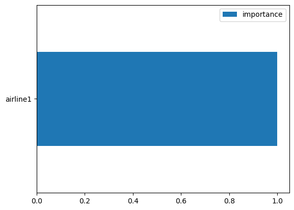
过去的变量重要性
feature_importances['Past variable importance over time'].mean().sort_values().plot(kind='barh')
未来变量的重要性
feature_importances['Future variable importance over time'].mean().sort_values().plot(kind='barh')
2.2 随时间变化的变量重要性
未来变量随时间的重要性
每个未来协变量在每个未来时间步的的重要性
df=feature_importances['Future variable importance over time']


fig, ax = plt.subplots(figsize=(20, 10))
bottom = np.zeros(len(df.index))
for col in df.columns:
    p = ax.bar(np.arange(-len(df),0), df[col].values, 0.6, label=col, bottom=bottom)
    bottom += df[col]
ax.set_title('Future variable importance over time ponderated by attention')
ax.set_ylabel("Importance")
ax.set_xlabel("Time")
ax.grid(True)
ax.legend()
plt.show()
请提供需要翻译的ipynb文件的具体内容,我将帮助您进行翻译。
随时间变化的过去变量重要性
df= feature_importances['Past variable importance over time']

fig, ax = plt.subplots(figsize=(20, 10))
bottom = np.zeros(len(df.index))

for col in df.columns:
    p = ax.bar(np.arange(-len(df),0), df[col].values, 0.6, label=col, bottom=bottom)
    bottom += df[col]
ax.set_title('Past variable importance over time')
ax.set_ylabel("Importance")
ax.set_xlabel("Time")
ax.legend()
ax.grid(True)

plt.show()
随时间变化的过去变量重要性,基于注意力进行加权
基于各时间步上变量的重要性,对每个时间步的重要性进行分解。
df= feature_importances['Past variable importance over time']
mean_attention = nf.models[0].attention_weights()[nf.models[0].input_size:,:].mean(axis=0)[:nf.models[0].input_size]
df = df.multiply(mean_attention, axis=0)

fig, ax = plt.subplots(figsize=(20, 10))
bottom = np.zeros(len(df.index))

for col in df.columns:
    p = ax.bar(np.arange(-len(df),0), df[col].values, 0.6, label=col, bottom=bottom)
    bottom += df[col]
ax.set_title('Past variable importance over time ponderated by attention')
ax.set_ylabel("Importance")
ax.set_xlabel("Time")
ax.legend()
ax.grid(True)
plt.plot(np.arange(-len(df),0), mean_attention, color='black', marker='o', linestyle='-', linewidth=2, label='mean_attention')
plt.legend()
plt.show()
3. 随时间变化的变量重要性相关性
在同一时刻获得和失去重要性的变量
nf.models[0].feature_importance_correlations()| trend | y_[lag12] | month | observed_target | Correlation with Mean Attention | |
|---|---|---|---|---|---|
| trend | 1.00 | -0.39 | -0.93 | 0.27 | 0.60 |
| y_[lag12] | -0.39 | 1.00 | 0.37 | -0.93 | -0.76 |
| month | -0.93 | 0.37 | 1.00 | -0.37 | -0.66 |
| observed_target | 0.27 | -0.93 | -0.37 | 1.00 | 0.77 |
| Correlation with Mean Attention | 0.60 | -0.76 | -0.66 | 0.77 | 1.00 |
Give us a ⭐ on Github