循环神经网络 (RNN)

%load_ext autoreload
%autoreload 2

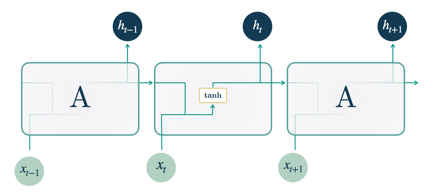
Elman在1990年提出了这一经典的递归神经网络（RNN），其中每一层使用以下递归变换： \[\mathbf{h}^{l}_{t} = \mathrm{Activation}([\mathbf{y}_{t},\mathbf{x}^{(h)}_{t},\mathbf{x}^{(s)}] W^{\intercal}_{ih} + b_{ih} + \mathbf{h}^{l}_{t-1} W^{\intercal}_{hh} + b_{hh})\]

其中，\(\mathbf{h}^{l}_{t}\) 是时间 \(t\) 下 RNN 层 \(l\) 的隐藏状态，\(\mathbf{y}_{t}\) 是时间 \(t\) 的输入，\(\mathbf{h}_{t-1}\) 是时间 \(t-1\) 的前一层的隐藏状态，\(\mathbf{x}^{(s)}\) 是静态外生输入，\(\mathbf{x}^{(h)}_{t}\) 是历史外生输入，\(\mathbf{x}^{(f)}_{[:t+H]}\) 是在预测时可用的未来外生输入。可用的激活函数有 tanh 和 relu。通过将隐藏状态转换成上下文 \(\mathbf{c}_{[t+1:t+H]}\) 来获得预测，这些上下文通过MLP解码并适应为 \(\mathbf{\hat{y}}_{[t+1:t+H],[q]}\)。

\[\begin{align} \mathbf{h}_{t} &= \textrm{RNN}([\mathbf{y}_{t},\mathbf{x}^{(h)}_{t},\mathbf{x}^{(s)}], \mathbf{h}_{t-1})\\ \mathbf{c}_{[t+1:t+H]}&=\textrm{Linear}([\mathbf{h}_{t}, \mathbf{x}^{(f)}_{[:t+H]}]) \\ \hat{y}_{\tau,[q]}&=\textrm{MLP}([\mathbf{c}_{\tau},\mathbf{x}^{(f)}_{\tau}]) \end{align}\]

参考文献
-Jeffrey L. Elman (1990). “在时间中寻找结构”.
-Cho, K., van Merrienboer, B., Gülcehre, C., Bougares, F., Schwenk, H., & Bengio, Y. (2014). 使用RNN编码器-解码器学习短语表示用于统计机器翻译.

图 1. 带有 MLP 解码器的单层 Elman RNN。

from nbdev.showdoc import show_doc
from neuralforecast.utils import generate_series

from typing import Optional

import torch
import torch.nn as nn

from neuralforecast.losses.pytorch import MAE
from neuralforecast.common._base_recurrent import BaseRecurrent
from neuralforecast.common._modules import MLP

class RNN(BaseRecurrent):
    """ RNN

    Multi Layer Elman RNN (RNN), with MLP decoder.
    The network has `tanh` or `relu` non-linearities, it is trained using 
    ADAM stochastic gradient descent. The network accepts static, historic 
    and future exogenous data.

    **Parameters:**<br>
    `h`: int, forecast horizon.<br>
    `input_size`: int, maximum sequence length for truncated train backpropagation. Default -1 uses all history.<br>
    `inference_input_size`: int, maximum sequence length for truncated inference. Default -1 uses all history.<br>
    `encoder_n_layers`: int=2, number of layers for the RNN.<br>
    `encoder_hidden_size`: int=200, units for the RNN's hidden state size.<br>
    `encoder_activation`: str=`tanh`, type of RNN activation from `tanh` or `relu`.<br>
    `encoder_bias`: bool=True, whether or not to use biases b_ih, b_hh within RNN units.<br>
    `encoder_dropout`: float=0., dropout regularization applied to RNN outputs.<br>
    `context_size`: int=10, size of context vector for each timestamp on the forecasting window.<br>
    `decoder_hidden_size`: int=200, size of hidden layer for the MLP decoder.<br>
    `decoder_layers`: int=2, number of layers for the MLP decoder.<br>
    `futr_exog_list`: str list, future exogenous columns.<br>
    `hist_exog_list`: str list, historic exogenous columns.<br>
    `stat_exog_list`: str list, static exogenous columns.<br>
    `loss`: PyTorch module, instantiated train loss class from [losses collection](https://nixtla.github.io/neuralforecast/losses.pytorch.html).<br>
    `valid_loss`: PyTorch module=`loss`, instantiated valid loss class from [losses collection](https://nixtla.github.io/neuralforecast/losses.pytorch.html).<br>
    `max_steps`: int=1000, maximum number of training steps.<br>
    `learning_rate`: float=1e-3, Learning rate between (0, 1).<br>
    `num_lr_decays`: int=-1, Number of learning rate decays, evenly distributed across max_steps.<br>
    `early_stop_patience_steps`: int=-1, Number of validation iterations before early stopping.<br>
    `val_check_steps`: int=100, Number of training steps between every validation loss check.<br>
    `batch_size`: int=32, number of differentseries in each batch.<br>
    `valid_batch_size`: int=None, number of different series in each validation and test batch.<br>
    `scaler_type`: str='robust', type of scaler for temporal inputs normalization see [temporal scalers](https://nixtla.github.io/neuralforecast/common.scalers.html).<br>
    `random_seed`: int=1, random_seed for pytorch initializer and numpy generators.<br>
    `num_workers_loader`: int=os.cpu_count(), workers to be used by `TimeSeriesDataLoader`.<br>
    `drop_last_loader`: bool=False, if True `TimeSeriesDataLoader` drops last non-full batch.<br>
    `optimizer`: Subclass of 'torch.optim.Optimizer', optional, user specified optimizer instead of the default choice (Adam).<br>
    `optimizer_kwargs`: dict, optional, list of parameters used by the user specified `optimizer`.<br>
    `lr_scheduler`: Subclass of 'torch.optim.lr_scheduler.LRScheduler', optional, user specified lr_scheduler instead of the default choice (StepLR).<br>
    `lr_scheduler_kwargs`: dict, optional, list of parameters used by the user specified `lr_scheduler`.<br>    
    `alias`: str, optional,  Custom name of the model.<br>

    `**trainer_kwargs`: int,  keyword trainer arguments inherited from [PyTorch Lighning's trainer](https://pytorch-lightning.readthedocs.io/en/stable/api/pytorch_lightning.trainer.trainer.Trainer.html?highlight=trainer).<br>    
    """
    # 类属性
    SAMPLING_TYPE = 'recurrent'
    EXOGENOUS_FUTR = True
    EXOGENOUS_HIST = True
    EXOGENOUS_STAT = True

    def __init__(self,
                 h: int,
                 input_size: int = -1,
                 inference_input_size: int = -1,
                 encoder_n_layers: int = 2,
                 encoder_hidden_size: int = 200,
                 encoder_activation: str = 'tanh',
                 encoder_bias: bool = True,
                 encoder_dropout: float = 0.,
                 context_size: int = 10,
                 decoder_hidden_size: int = 200,
                 decoder_layers: int = 2,
                 futr_exog_list = None,
                 hist_exog_list = None,
                 stat_exog_list = None,
                 loss = MAE(),
                 valid_loss = None,
                 max_steps: int = 1000,
                 learning_rate: float = 1e-3,
                 num_lr_decays: int = -1,
                 early_stop_patience_steps: int =-1,
                 val_check_steps: int = 100,
                 batch_size=32,
                 valid_batch_size: Optional[int] = None,
                 scaler_type: str='robust',
                 random_seed=1,
                 num_workers_loader=0,
                 drop_last_loader=False,
                 optimizer=None,
                 optimizer_kwargs=None,
                 lr_scheduler = None,
                 lr_scheduler_kwargs = None,                 
                 **trainer_kwargs):
        super(RNN, self).__init__(
            h=h,
            input_size=input_size,
            inference_input_size=inference_input_size,
            loss=loss,
            valid_loss=valid_loss,
            max_steps=max_steps,
            learning_rate=learning_rate,
            num_lr_decays=num_lr_decays,
            early_stop_patience_steps=early_stop_patience_steps,
            val_check_steps=val_check_steps,
            batch_size=batch_size,
            valid_batch_size=valid_batch_size,
            scaler_type=scaler_type,
            futr_exog_list=futr_exog_list,
            hist_exog_list=hist_exog_list,
            stat_exog_list=stat_exog_list,
            num_workers_loader=num_workers_loader,
            drop_last_loader=drop_last_loader,
            random_seed=random_seed,
            optimizer=optimizer,
            optimizer_kwargs=optimizer_kwargs,
            lr_scheduler=lr_scheduler,
            lr_scheduler_kwargs=lr_scheduler_kwargs,
            **trainer_kwargs
        )

        # 循环神经网络
        self.encoder_n_layers = encoder_n_layers
        self.encoder_hidden_size = encoder_hidden_size
        self.encoder_activation = encoder_activation
        self.encoder_bias = encoder_bias
        self.encoder_dropout = encoder_dropout
        
        # 上下文适配器
        self.context_size = context_size

        # 多层感知器解码器
        self.decoder_hidden_size = decoder_hidden_size
        self.decoder_layers = decoder_layers

        # 循环神经网络 输入大小（1 表示目标变量 y）
        input_encoder = 1 + self.hist_exog_size + self.stat_exog_size

        # 实例化模型
        self.hist_encoder = nn.RNN(input_size=input_encoder,
                                   hidden_size=self.encoder_hidden_size,
                                   num_layers=self.encoder_n_layers,
                                   nonlinearity=self.encoder_activation,
                                   bias=self.encoder_bias,
                                   dropout=self.encoder_dropout,
                                   batch_first=True)

        # 上下文适配器
        self.context_adapter = nn.Linear(in_features=self.encoder_hidden_size + self.futr_exog_size * h,
                                         out_features=self.context_size * h)

        # 解码器多层感知机
        self.mlp_decoder = MLP(in_features=self.context_size + self.futr_exog_size,
                               out_features=self.loss.outputsize_multiplier,
                               hidden_size=self.decoder_hidden_size,
                               num_layers=self.decoder_layers,
                               activation='ReLU',
                               dropout=0.0)

    def forward(self, windows_batch):
        
        # 解析Windows批处理文件
        encoder_input = windows_batch['insample_y'] # [B, 序列长度, 1]
        futr_exog     = windows_batch['futr_exog']
        hist_exog     = windows_batch['hist_exog']
        stat_exog     = windows_batch['stat_exog']

        # 连接y、历史输入和静态输入
        # [B, C, seq_len, 1] -> [B, seq_len, C]
        # 连接 [ Y_t, | X_{t-L},..., X_{t} | S ]
        batch_size, seq_len = encoder_input.shape[:2]
        if self.hist_exog_size > 0:
            hist_exog = hist_exog.permute(0,2,1,3).squeeze(-1) # [B, X, seq_len, 1] -> [B, seq_len, X]
            encoder_input = torch.cat((encoder_input, hist_exog), dim=2)

        if self.stat_exog_size > 0:
            stat_exog = stat_exog.unsqueeze(1).repeat(1, seq_len, 1) # [B, S] -> [B, seq_len, S]
            encoder_input = torch.cat((encoder_input, stat_exog), dim=2)

        # 循环神经网络 前向传播
        hidden_state, _ = self.hist_encoder(encoder_input) # [B, seq_len, rnn_隐藏状态]

        if self.futr_exog_size > 0:
            futr_exog = futr_exog.permute(0,2,3,1)[:,:,1:,:]  # [B, F, seq_len, 1+H] -> [B, seq_len, H, F]
            hidden_state = torch.cat(( hidden_state, futr_exog.reshape(batch_size, seq_len, -1)), dim=2)

        # 上下文适配器
        context = self.context_adapter(hidden_state)
        context = context.reshape(batch_size, seq_len, self.h, self.context_size)

        # 带有未来外部变量的残差连接
        if self.futr_exog_size > 0:
            context = torch.cat((context, futr_exog), dim=-1)

        # 最终预测
        output = self.mlp_decoder(context)
        output = self.loss.domain_map(output)
        
        return output

show_doc(RNN)

show_doc(RNN.fit, name='RNN.fit')

show_doc(RNN.predict, name='RNN.predict')

使用示例

import pandas as pd
import matplotlib.pyplot as plt

from neuralforecast import NeuralForecast
from neuralforecast.models import RNN
from neuralforecast.losses.pytorch import MQLoss, DistributionLoss
from neuralforecast.utils import AirPassengersPanel, AirPassengersStatic

Y_train_df = AirPassengersPanel[AirPassengersPanel.ds<AirPassengersPanel['ds'].values[-12]] # 132次列车
Y_test_df = AirPassengersPanel[AirPassengersPanel.ds>=AirPassengersPanel['ds'].values[-12]].reset_index(drop=True) # 12项测试

fcst = NeuralForecast(
    models=[RNN(h=12,
                input_size=-1,
                inference_input_size=24,
                loss=MQLoss(level=[80, 90]),
                scaler_type='robust',
                encoder_n_layers=2,
                encoder_hidden_size=128,
                context_size=10,
                decoder_hidden_size=128,
                decoder_layers=2,
                max_steps=300,
                futr_exog_list=['y_[lag12]'],
                #hist_exog_list=['y_[lag12]'],
                stat_exog_list=['airline1'],
                )
    ],
    freq='M'
)
fcst.fit(df=Y_train_df, static_df=AirPassengersStatic, val_size=12)
forecasts = fcst.predict(futr_df=Y_test_df)

Y_hat_df = forecasts.reset_index(drop=False).drop(columns=['unique_id','ds'])
plot_df = pd.concat([Y_test_df, Y_hat_df], axis=1)
plot_df = pd.concat([Y_train_df, plot_df])

plot_df = plot_df[plot_df.unique_id=='Airline1'].drop('unique_id', axis=1)
plt.plot(plot_df['ds'], plot_df['y'], c='black', label='True')
plt.plot(plot_df['ds'], plot_df['RNN-median'], c='blue', label='median')
plt.fill_between(x=plot_df['ds'][-12:], 
                 y1=plot_df['RNN-lo-90'][-12:].values, 
                 y2=plot_df['RNN-hi-90'][-12:].values,
                 alpha=0.4, label='level 90')
plt.legend()
plt.grid()
plt.plot()

Give us a ⭐ on Github